Relativistic quantum mechanics 2nd edition

Texts and Monographs in Physics
Series Editors:
R. Balian, Gif-sur-Yvette, France
W. Beiglböck, Heidelberg, Germany
H. Grosse, Wien, Austria
W. Thirring, Wien, Austria


Hartmut M. Pilkuhn

Relativistic
Quantum Mechanics
Second Edition
With 21 Figures

123
www.pdfgrip.com


Professor Hartmut M. Pilkuhn
Universität Karlsruhe
Institut für theoretische Teilchenphysik
76128 Karlsruhe, Germany
e-mail:

Library of Congress Control Number: 2005929195

ISSN 0172-5998
ISBN-10 3-540-25502-8 2nd ed. Springer Berlin Heidelberg New York
ISBN-13 978-3-540-25502-4 2nd ed.Springer Berlin Heidelberg New York
ISBN 3-540-43666-9 1st ed. Springer-Verlag Berlin Heidelberg New York

This work is subject to copyright. All rights are reserved, whether the whole or part of the material is concerned,
specifically the rights of translation, reprinting, reuse of illustrations, recitation, broadcasting, reproduction on microfilm
or in any other way, and storage in data banks. Duplication of this publication or parts thereof is permitted only under
the provisions of the German Copyright Law of September 9, 1965, in its current version, and permission for use must
always be obtained from Springer. Violations are liable for prosecution under the German Copyright Law.
Springer is a part of Springer Science+Business Media
springeronline.com
c Springer-Verlag Berlin Heidelberg 2003, 2005
Printed in Germany
The use of general descriptive names, registered names, trademarks, etc. in this publication does not imply, even in the
absence of a specific statement, that such names are exempt from the relevant probreak tective laws and regulations and
therefore free for general use.
Typesetting: Data conversion by LE-TeX Jelonek, Schmidt & Vöckler GbR
Cover design: design & production GmbH, Heidelberg
Printed on acid-free paper SPIN 11414094 55/3141/YL 5 4 3 2 1 0

www.pdfgrip.com


Preface to the Second Edition

This edition includes five new sections and a third appendix. Most other sections are expanded, in particular Sects. 5.2 and 5.6 on hyperfine interactions.
Section 3.8 offers an introduction to the important field of relativistic
quantum chemistry. In Sect. 5.7, the coupling of the anomalous magnetic
moment is needed for a relativistic treatment of the proton in hydrogen. It
generalizes a remarkable feature of leptonium, namely the non-hermiticity of
magnetic hyperfine interactions. In Appendix C, the explicit calculation of
the expectation value of an operator which is frequently approximated by
a delta-function confirms that the singularity of relativistic wave functions at
the origin is correct.

The other three new sections cover dominantly nonrelaticistic topics, in
particular the quark model. The coupling of three electron spins (Sect. 3.9)
provides also the basis for the three quark spins of baryons (Sect. 5.9). For less
than four particles, direct symmetry arguments are simpler than the representions of the permutation group which are normally used in the literature.
Another new topic of this edition is the confirmation of the E 2 -dependence
of atomic equations by the relativistic energy conservation in radiative atomic
transitions, according to the time-dependent perturbation theory of Sect. 5.4.
In the quark model, the E 2 -theorem applies not only to mesons, but also to
baryons as three-quark bound states. Unfortunately, the non-existence of free
quarks prevents a precise formulation of the phenomenological “constituent
quark model”, which remains the most challenging problem of relativistic
quantum mechanics.
Karlsruhe, May 2005

Hartmut M. Pilkuhn

www.pdfgrip.com


Preface

Whereas nonrelativistic quantum mechanics is sufficient for any understanding of atomic and molecular spectra, relativistic quantum mechanics explains
the finer details. Consequently, textbooks on quantum mechanics expand
mainly on the nonrelativistic formalism. Only the Dirac equation for the
hydrogen atom is normally included. The relativistic quantum mechanics
of one- and two-electron atoms is covered by Bethe and Salpeter (1957),
Mizushima (1970) and others. Books with emphasis on atomic and molecular
applications discuss also effective “first-order relativistic” operators such as
spin-orbit coupling, tensor force and hyperfine operators (Weissbluth 1978).
The practical importance of these topics has led to specialized books, for

example that of Richards, Trivedi and Cooper (1981) on spin-orbit coupling
in molecules, or that of Das (1987) on the relativistic quantum mechanics of
electrons. The further development in this direction is mainly the merit of
quantum chemists, normally on the basis of the multi-electron Dirac-Breit
equation. The topic is covered in reviews (Lawley 1987, Wilson et al. 1991);
an excellent monograph by Strange (1998) includes solid-state theory.
Relativistic quantum mechanics is an application of quantum field theory
to systems with a given number of massive particles. This is not easy, since
the basic field equations (Klein-Gordon and Dirac) contain creation and annihilation operators that can produce unphysical negative-energy solutions in
the derived single-particle equations. However, one has learned how to handle these states, even in atoms with two or more electrons. The methods are
not particularly elegant; residual problems will be mentioned at the end of
Chap. 3. But even there, the precision of these methods is impressive. For example, the influence of virtual electron-positron pairs is included by vacuum
polarization, in the form of the Uehling, Kroll-Wichman and Kă
allen-Sabry
potentials (Sect. 5.3). For two-body problems, improved methods allow for
a fantastic precision, which provides by far the most accurate test of quantum electrodynamics itself.
The present book introduces quantum mechanics in analogy with the
Maxwell equations rather than classical mechanics; it emphasizes Lorentz
invariance and treats the nonrelativistic version as an approximation. The
important quantum field is the photon field, i.e. the electromagnetic field in
the Coulomb gauge, but fields for massive particles are also needed. On the

www.pdfgrip.com


VIII

Preface

other hand, the presentation is very different from that of books on quantum field theory, which include preparatory chapters on classical fields and

relativistic quantum mechanics (for example Gross 1993, Yndurain 1996).
The Coulomb gauge is mandatory not only for atomic spectra, but also
for the related “quark model” calculations of baryon spectra, which form
an important part of the theory of strong interactions. A by-product of an
entirely relativistic bound state formalism is a twofold degenerate spectrum,
due to explicit charge conjugation invariance. Quark model calculations might
benefit from such relatively simple improvements, even when the spectra may
eventually be calculated “on the lattice”.
A new topic of this book is a rather broad formalism for relativistic
two-body (“binary”) atoms: Nonrelativistically, the Schră
odinger equation for
an isolated binary can be reduced to an equivalent one-body equation, in
which the electron mass is replaced by the “reduced mass”. The extension of
this treatment to two relativistic particles will be explained in Chap. 4. The
case of two spinless particles was solved already in 1970, see the introduction to Sect. 4.5. The much more important “leptonium” case is treated in
Sects. 4.6 and 4.7.
Stimulated by the enormous success of the single-particle Dirac equation, Bethe and Salpeter (1951) constructed a sixteen-component equation
for two-fermion binaries. However, increasingly precise calculations disclosed
weak points. An effective Dirac equation with a reduced mass cannot be
derived from a sixteen-component equation except by an approximate “quasidistance” transformation. On the other hand, such a Dirac equation does
follow very directly in an eight-component formalism, in which the relevant
S-matrix is prepared as an 8 × 8-matrix. The principle will be explained in
Sect. 4.6, the interaction is added in Sect. 4.7. Like in the Schrăodinger equation with reduced mass, the coupling to the photon vector potential operator
is treated perturbatively. The famous “Lamb shift” calculation will be presented in Sect. 5.5, extended to the two-body case.
A remarkable property of the new binary equations is the absence of “retardation”. Its disappearance will be demonstrated in Sect. 4.9. Most fermions
have an inner structure which requires extra operators already in the singleparticle equation. As an example, the fine structure of antiprotonic atoms
will be discussed in Sect. 5.6. The Uehling potential is also detailed for these
and other “exotic” atoms.
Preparatory studies for this book have been supported by the Volkswagenstiftung. The book would have been impossible without the efforts of my
students and collaborators, B. Melic and R. Hăackl, M. Malvetti and V. Hund.

A textbook by Hund, Malvetti and myself (1997) has provided some of its
material.
I dedicate this book to the memory of Oskar Klein.
Karlsruhe, March 2002

Hartmut M. Pilkuhn

www.pdfgrip.com


Contents

1

Maxwell and Schră
odinger . . . . . . . . . . . . . . . . . . . . . . . . . . . . . . . . .
1.1 Light and Linear Operators . . . . . . . . . . . . . . . . . . . . . . . . . . . . . .
1.2 De Broglies Idea and Schrăodingers Equation . . . . . . . . . . . . . . .
1.3 Potentials and Gauge Invariance . . . . . . . . . . . . . . . . . . . . . . . . . .
1.4 Stationary Potentials, Zeeman Shifts . . . . . . . . . . . . . . . . . . . . . .
1.5 Bound States . . . . . . . . . . . . . . . . . . . . . . . . . . . . . . . . . . . . . . . . . .
1.6 Spinless Hydrogenlike Atoms . . . . . . . . . . . . . . . . . . . . . . . . . . . . .
1.7 Landau Levels and Harmonic Oscillator . . . . . . . . . . . . . . . . . . .
1.8 Orthogonality and Measurements . . . . . . . . . . . . . . . . . . . . . . . . .
1.9 Operator Methods, Matrices . . . . . . . . . . . . . . . . . . . . . . . . . . . . .
1.10 Scattering and Phase Shifts . . . . . . . . . . . . . . . . . . . . . . . . . . . . . .

1
1
5

9
13
16
20
26
30
38
49

2

Lorentz, Pauli and Dirac . . . . . . . . . . . . . . . . . . . . . . . . . . . . . . . . . .
2.1 Lorentz Transformations . . . . . . . . . . . . . . . . . . . . . . . . . . . . . . . .
2.2 Spinless Current, Density of States . . . . . . . . . . . . . . . . . . . . . . .
2.3 Pauli’s Electron Spin . . . . . . . . . . . . . . . . . . . . . . . . . . . . . . . . . . . .
2.4 The Dirac Equation . . . . . . . . . . . . . . . . . . . . . . . . . . . . . . . . . . . .
2.5 Addition of Angular Momenta . . . . . . . . . . . . . . . . . . . . . . . . . . .
2.6 Hydrogen Atom and Parity Basis . . . . . . . . . . . . . . . . . . . . . . . . .
2.7 Alternative Form, Perturbations . . . . . . . . . . . . . . . . . . . . . . . . . .
2.8 The Pauli Equation . . . . . . . . . . . . . . . . . . . . . . . . . . . . . . . . . . . . .
2.9 The Zeeman Effect . . . . . . . . . . . . . . . . . . . . . . . . . . . . . . . . . . . . .
2.10 The Dirac Current. Free Electrons . . . . . . . . . . . . . . . . . . . . . . . .

53
53
57
60
66
71
75

82
89
94
98

3

Quantum Fields and Particles . . . . . . . . . . . . . . . . . . . . . . . . . . . .
3.1 The Photon Field . . . . . . . . . . . . . . . . . . . . . . . . . . . . . . . . . . . . . .
3.2 C, P and T . . . . . . . . . . . . . . . . . . . . . . . . . . . . . . . . . . . . . . . . . . . .
3.3 Field Operators and Wave Equations . . . . . . . . . . . . . . . . . . . . .
3.4 Breit Operators . . . . . . . . . . . . . . . . . . . . . . . . . . . . . . . . . . . . . . . .
3.5 Two-Electron States and Pauli Principle . . . . . . . . . . . . . . . . . . .
3.6 Elimination of Components . . . . . . . . . . . . . . . . . . . . . . . . . . . . . .
3.7 Brown-Ravenhall Disease, Energy Projectors,
Improved Breitian . . . . . . . . . . . . . . . . . . . . . . . . . . . . . . . . . . . . . .
3.8 Variational Method, Shell Model . . . . . . . . . . . . . . . . . . . . . . . . .
3.9 The Pauli Principle for Three Electrons . . . . . . . . . . . . . . . . . . .

103
103
108
113
118
121
126

www.pdfgrip.com

132

136
141


X

Contents

4

Scattering and Bound States . . . . . . . . . . . . . . . . . . . . . . . . . . . . .
4.1 Introduction . . . . . . . . . . . . . . . . . . . . . . . . . . . . . . . . . . . . . . . . . . .
4.2 Born Series and S-Matrix . . . . . . . . . . . . . . . . . . . . . . . . . . . . . . . .
4.3 Two-body Scattering and Decay . . . . . . . . . . . . . . . . . . . . . . . . . .
4.4 Current Matrix Elements, Form Factors . . . . . . . . . . . . . . . . . . .
4.5 Particles of Higher Spins . . . . . . . . . . . . . . . . . . . . . . . . . . . . . . . .
4.6 The Equation for Spinless Binaries . . . . . . . . . . . . . . . . . . . . . . . .
4.7 The Leptonium Equation . . . . . . . . . . . . . . . . . . . . . . . . . . . . . . . .
4.8 The Interaction in Leptonium . . . . . . . . . . . . . . . . . . . . . . . . . . . .
4.9 Binary Boosts . . . . . . . . . . . . . . . . . . . . . . . . . . . . . . . . . . . . . . . . . .
4.10 Klein-Dirac Equation, Hydrogen . . . . . . . . . . . . . . . . . . . . . . . . . .
4.11 Dirac Structures of Binary Bound States . . . . . . . . . . . . . . . . . .

143
143
144
150
159
165
168

174
178
184
190
196

5

Hyperfine Shifts, Radiation, Quarks . . . . . . . . . . . . . . . . . . . . . .
5.1 First-Order Magnetic Hyperfine Splitting . . . . . . . . . . . . . . . . . .
5.2 Nonrelativistic Magnetic Hyperfine Operators . . . . . . . . . . . . . .
5.3 Vacuum Polarization, Dispersion Relations . . . . . . . . . . . . . . . .
5.4 Atomic Radiation . . . . . . . . . . . . . . . . . . . . . . . . . . . . . . . . . . . . . .
5.5 Soft Photons, Lamb Shift . . . . . . . . . . . . . . . . . . . . . . . . . . . . . . . .
5.6 Antiprotonic Atoms, Quadrupole Potential . . . . . . . . . . . . . . . .
5.7 The Magnetic Moment Interaction . . . . . . . . . . . . . . . . . . . . . . . .
5.8 SU2 , SU3 , Quarks . . . . . . . . . . . . . . . . . . . . . . . . . . . . . . . . . . . . . .
5.9 Baryon Magnetic Moments . . . . . . . . . . . . . . . . . . . . . . . . . . . . . .

201
201
206
211
219
225
232
239
243
250

A

Orthonormality and Expectation Values . . . . . . . . . . . . . . . . . . 253

B

Coulomb Greens Functions . . . . . . . . . . . . . . . . . . . . . . . . . . . . . . . 259

C

Yukawa Expectation Values . . . . . . . . . . . . . . . . . . . . . . . . . . . . . . . 261

Bibliography . . . . . . . . . . . . . . . . . . . . . . . . . . . . . . . . . . . . . . . . . . . . . . . . . . 267
Index . . . . . . . . . . . . . . . . . . . . . . . . . . . . . . . . . . . . . . . . . . . . . . . . . . . . . . . . . 273

www.pdfgrip.com


1 Maxwell and Schră
odinger

1.1 Light and Linear Operators
Electromagnetic radiation is classified according to wavelength in radio and
microwaves, infrared, visible and UV light, X- and Gamma rays. These names
indicate that the particle aspect of the radiation dominates at short wavelengths, while the wave aspect dominates at long wavelengths. Nevertheless,
the radiation is described at all wavelengths by electric and magnetic fields,
E and B, which obey wave equations. The quantum aspects of these fields
will be discussed in Chap. 3. In vacuum, the equation for E is
(−c−2 ∂t2 + ∂x2 + ∂y2 + ∂z2 )E = 0,

∂t = ∂/∂t, ∂x = ∂/∂x,

(1.1)

where c = 299 792 458 m/s is the velocity of light in vacuum. For the time
being, we are mainly interested in the form of this dierential equation, which
guided Schră
odinger in the construction of his equation for electrons. In vectorial notation, r = (x, y, z) is the position vector, and ∇ = (∂x , ∂y , ∂z ) =
“nabla” is the gradient vector; its square is the Laplacian ∆. Particularly in
relativistic context, one prefers the notation xi = (x1 , x2 , x3 ) = (x, y, z):
3

∇2 = ∆ = ∂x2 + ∂y2 + ∂z2 =

∂i2 ,

∂i ≡ ∂/∂xi .

(1.2)

i=1

The xi is conveniently combined with x0 = ct into a four-vector xµ =
(x0 , xi ) = (x0 , r), and the −c2 ∂t2 of (1.1) is combined with ∇2 into the
d’Alembertian operator , also called “quabla”:
E = 0;

= −∂02 + ∇2 ,

∂0 = ∂/∂(ct).

(1.3)

The full use of this nomenclature will be postponed to Chap. 2. For the moment, t is expressed in terms of x0 merely to suppress the constant c. Today,
c is in fact used in the definition of the length scale, see Sect. 1.6.
Differential operators D are linear in the sense D(E 1 +E 2 ) = DE 1 +DE2 .
If E 1 and E 2 are two different solutions of (1.1), E = E 1 + E 2 is a third
one. This is called the superposition principle. The intensity I of light is
normally measured by E 2 , I ∼ E 2 ≡ square(E), but nonlinear operators such as “square” are not used in quantum mechanics. ∇ and ∇2 are

www.pdfgrip.com


2

1 Maxwell and Schră
odinger
z

y




x

Fig. 1.1. Cylinder coordinates

both linear operators. The simplest operator is a multiplicative constant
C, C(E 1 + E 2 ) = CE 1 + CE 2 . We now recall some operators of classical

electrodynamics, which will be needed in quantum mechanics. The Laplacian
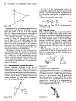
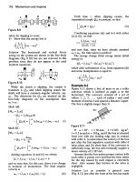
is in cylindrical coordinates (Fig. 1.1)
x = ρ cos φ, y = ρ sin φ,

(1.4)

∇2 = ∂z2 + ρ−1 ∂ρ ρ∂ρ + ρ−2 ∂φ2 ,

(1.5)

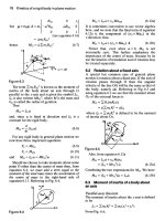
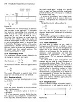
and in spherical coordinates (Fig. 1.2):
z = r cos θ, ρ = r sin θ,

(1.6)

∇2 = r−1 ∂r2 r + r−2 (r × ∇)2 .

(1.7)

r × ∇ is somewhat complicated, but its z-component is simple:
(r × ∇)z = x∂y − y∂x = ∂φ .

(1.8)

The square of r × ∇ is also relatively simple,
(r × ∇)2 = ∂φ2 (1 − u2 )−1 + ∂u (1 − u2 )∂u ,

u = cos θ.

(1.9)

Two operators A and B are said to commute if the order in which they are
applied to the wave function does not matter, AB = BA. For example, as
r × ∇ depends only on θ and φ, not on r, one has r−2 (r × ∇)2 = (r × ∇)2 r−2 .
On the other hand, in the radial part r−1 ∂r2 r of the Laplacian (1.7), the first
z

r
ϑ
y

ϕ
x

ρ

Fig. 1.2. Spherical coordinates

www.pdfgrip.com


1.1 Light and Linear Operators

3

two operators do not commute, r−1 ∂r2 = ∂r2 r−1 (otherwise one would have
r−1 ∂r2 r = ∂r2 ). Valid alternative forms are
r−1 ∂r2 r = (∂r + 1/r)2 = ∂r2 + 2r−1 ∂r .

(1.10)

To check these, apply the operators to an arbitrary function f (r) and use
∂r f (r) = f (r), ∂r f g = f g + f g , (∂r + 1/r)2 = (∂r + 1/r)(∂r + 1/r).
Equation (1.1) has plane-wave solutions of the type
E = E 0 eikr−iωt ,

ω = 2πν.

(1.11)

k = (kx , ky , kz ),

λ = 2π/k,

(1.12)

where k is the wave number vector, pointing into the direction of propagation
of the plane wave, and λ is the wavelength. Insertion of
∂t E = −iωE,

∂z E = ikz E, . . .

(1.13)

shows that (1.11) is a solution of the wave equation (1.1) only for
ω 2 /c2 = k2 = kx2 + ky2 + kz2 .

(1.14)

We shall also need cylindrical and spherical waves, where ∇2 is required in the

forms (1.5) and (1.7). Such waves can also be monochromatic, meaning that
they contain only one (angular) frequency ω. The common wave equation for
all monochromatic waves in vacuum is
E(xµ ) = e−iωt E ω (r),

(ω 2 /c2 + ∇2 )E ω (r) = 0.

(1.15)

This “Helmholtz equation” is still a partial differential equation in three
variables; we recall a few tricks for the solution of such equations. The main
trick is to express ∇2 in terms of commuting operators A, B, C, and then to
construct “eigenfunctions” of these operators. When A is applied to any of
its eigenfunctions fn , it may be replaced simply by a constant an , called the
eigenvalue:
Afn = an fn .
(1.16)
For example, the square of the operator ∂φ occurs both in cylindrical and
in spherical coordinates. The normalized eigenfunctions of ∂φ are
ψml (φ) = (2π)−1/2 eiml φ ,

ml = 0, ±1, ±2 . . .

(1.17)

In quantum mechanics, ml is called the (orbital) magnetic quantum number
(Sect. 1.4). The normalization is chosen such that
2π
0

∗
ψm
ψ dφ =
l ml

2π
0

|ψml |2 dφ = 1.

www.pdfgrip.com

(1.18)


4

1 Maxwell and Schră
odinger

It xes the scale of the eigenfunction. An essential point of (1.17) is the
restriction of the eigenvalues ml of −i∂φ to integer values, due to the required
single-valuedness of ψ at all φ:
ψml (φ + 2π) = ψml (φ).

(1.19)

For such eigenfunctions, one may replace the operator ∂φ2 by one of its eigenvalues −m2l in the operators (1.5) or (1.9). For commuting operators A and
B there exist common eigenfunctions,
Afan ,bm = an fan ,bm , Bfan ,bm = bm fan ,bm ,

(1.20)

because ABf = BAf = an Bf shows that Bf is also an eigenfunction of A,
again with eigenvalue an . A rather trivial example of common eigenfunctions
is given by the plane waves (1.11), which are eigenfunctions of ∂x , ∂y , ∂z ,
with eigenvalues ikx , iky , ikz respectively. A famous example in spherical coordinates are the “spherical harmonics” Ylm (θ, φ) (with simplified notation
ml ≡ m), which are not only eigenfunctions of ∂φ , but also of (r × ∇)2 as
given by (1.9):
Ylm (θ, φ) = Θlm (θ)ψm (φ),
(1.21)
(r × ∇)2 Ylm = −l(l + 1)Ylm ,

− l ≤ m ≤ l.

l = 0, 1, 2 . . .

(1.22)

Θlm is a polynomial of degree |m| in sin θ and degree l − |m| in u = cos θ.
Some of these functions are collected in Table 1.1.
The Θl0 are Legendre polynomials Pl , apart from a normalization constant:
1

Θl0 = (l + 12 ) 2 Pl (u). P0 = 1, P1 = u, P2 = 12 (3u3 − 1), P3 = 12 (5u3 − 3u).
(1.23)
When applied to the spherical harmonics, the Laplacian (1.6) effectively becomes a radial operator, i.e. independent of θ and φ. Thus E ω (r) has solutions
of the form
E ω (r) = E 0 (ω)Rω,l (r)Ylm (θ, φ),
(1.24)

(ω 2 /c2 + ∇2 )E ω = E 0 Ylm [ω 2 /c2 + (∂r + 1/r)2 − l(l + 1)/r2 ]Rω,l (r). (1.25)
Table 1.1. Ylm for l < 3. Normalization (1.186), x± = ∓x − iy.
1

Y00

= (4π)− 2 ,

Y10

= (3/4π) 2 cos θ = (3/4π) 2 z/r,

1

1

1

1

Y1±1 = ∓(3/8π) 2 sin θe±iφ = (3/8π) 2 x± /r,
Y20

1

1

= (5/16π) 2 (3 cos2 θ − 1) = (5/16π) 2 (2z 2 + x+ x− )/r2 ,
1

1

Y2±1 = ∓(15/8π) 2 cos θ sin θe±iφ = (15/8π) 2 x± z/r2 ,
Y2±2 =

1
(15/32π) 2 e±2iφ

sin2 θ =

1
(15/32π) 2 x2± /r2 .

www.pdfgrip.com


1.2 De Broglies Idea and Schră
odingers Equation

5

Dividing o the rst two factors, one finds the differential equation for the
radial wave function R(r),
[ω 2 /c2 + (∂r + 1/r)2 − l(l + 1)/r2 ]Rω,l (r) = 0.

(1.26)

Also this equation has simple solutions, to be discussed in Sect. 1.10.
E need not be an eigenfunction of any of these operators, but it may be
expanded in terms of the eigenfunctions. Real light has a “spectral decomposition”,

∞

E(t, r) =

dωE ω (r)e−iωt ,

(1.27)

0

which expresses a wave train (or wave packet) as a superposition of monochromatic waves. Similarly, there will be a double integral over the directions of k
in (1.11), or equivalently a sum over l and m in (1.24). As a simple example
of a summation, consider a wave in a waveguide along the z-axis. The walls
of the waveguide in the x- and y-planes require standing waves along these
directions, of the form sin(kx x) sin(ky y). But
sin(kx x) = (2i)−1 eikx x − (2i)−1 e−ikx x

(1.28)

displays a standing wave as a superposition of two counterpropagating plane
waves. This also demonstrates that ∇2 has real eigenfunctions. The solution
(1.28) is an eigenfunction of ∂x2 , even though it is not an eigenfunction of ∂x .
Similarly, the spherical harmonics are only complex because we insisted on
using eigenfunctions of ∂φ in (1.17), where sin φ and cos φ would have been
equally possible from the point of view of ∂φ2 .
We conclude with the solution of (1.26) for l = 0, [ω 2 /c2 + (∂r +
1/r)2 ]Rω,0 (r) = 0. Also this equation has two solutions,
R± = r−1 e±ikr ,

(∂r + 1/r)R± = r−1 ∂r e±ikr = ±ikR± ,

(1.29)

with k2 = ω 2 /c2 , as usual. R+ is the simplest example of an outgoing spherical
wave. (It does not represent dipole radiation, because the Coulomb gauge
condition divE = 0 has been ignored.) For complex E, the intensity is I ∼
E ∗ E instead of E 2 . It decreases with r as r2 , as expected.

1.2 De Broglies Idea and Schră
odingers Equation
Although light does propagate according to the wave equation just discussed, it is nevertheless emitted and absorbed in quanta called photons.
In monochromatic light of the type (1.15), each photon has the same energy
E = hν, and in the case of a plane monochromatic wave (1.11), it also has
a fixed momentum p = hk/2π:
p=h
¯ k,

(1.30)

¯h = h/2π = 6.58218 × 10−16 eV s,

(1.31)

E = hν = h
¯ ω = hc/λ,

www.pdfgrip.com


6

1 Maxwell and Schră
odinger

where h is Plancks constant. The constants c and h
¯ (“hbar”) are so fundamental in relativistic quantum mechanics that they are often taken as natural
units (Sect. 1.6). On the basis of (1.30), Einstein (1905) translated the relation
ω 2 /c2 = k2 into an energy-momentum relation for photons,
E 2 /c2 = p2 .

(1.32)

For massive particles, he had to reconcile Newton’s expression EN = p2 /2m
(m = particle mass, p = mv) with his photon formula (1.32). As Newtonian
mechanics fixes EN only up to a constant, Einstein put E = mc2 + EN
and interpreted this expression as an approximation for small p/mc of the
function
E/c =

m2 c2 + p2 = mc + p2 /2mc − p4 /8m3 c3 ± . . .

(1.33)

He thus postulated the energy-momentum relation
E 2 /c2 − p2 = m2 c2

(1.34)

for all kinds of particles (including composite ones and even watches), and
obtained (1.32) as a special case for zero-mass particles. It may also be noted

that for p/mc > 1, the expansion (1.33) of the square root diverges. Instead,
the expansion in terms of mc/p < 1 is now convergent:
E/c = p + m2 c2 /2p − m4 c4 /8p3 ± . . .

(1.35)

Comparing with the E/c = p of (1.32), one may say that all particles of large
momenta mc/p ≈ 0 move also with the speed of light. There exist weakly interacting particles called neutrinos, which appear in beta decay. Their masses
are not exactly zero, but are neglible in all terrestrial experiments, such that
neutrinos move with the speed of light. In cosmic rays, electrons, protons
and even heavier nuclei sometimes move with the speed of light, too. For
most experiments, however, the system’s total energy E is close to i mi c2 ,
where the sum includes all particles which are explicitly considered. Even in
a fully relativistic calculation, it is often practical to subtract this constant.
Let us call the remaining energy EN in honour of Newton, even when the
calculation is relativistic. For example, when the energy levels of alkali atoms
are approximated by a single-electron model, one sets
E = me c2 + EN ,

me c2 = 510.9989 keV.

(1.36)

Already before the discovery of quantum mechanics, Rydberg found an empirical formula for EN ,
EN (n, l) = −R∞ /(n−β)2 ≡ −R∞ /n2β ,

n = 1, 2, 3 . . . , R∞ = 13.605691 eV.
(1.37)

www.pdfgrip.com

1.2 De Broglies Idea and Schră
odingers Equation

7

R is the Rydberg constant for an infinitely heavy nucleus, n is the principal quantum number, nβ the “effective” principal quantum number, (also
denoted by n∗ ), and β = β(l, n) is a “quantum defect” at orbital angular
momentum l (1.22). In alkali atoms, β > 0 is relatively large at small l where
the valence electron sees an increasing fraction of the nuclear charge Ze inside the screening charge cloud of the other electrons. (Actually, n = 1 exists
only for atomic hydrogen, which was studied later. Lithium (Z = 3) begins
with n = 2, sodium (Na, Z = 11) with n = 3, see Sect. 3.8. The other two
electrons of Li occupy the n = 1 “shell” which is “closed” according to Pauli
(1925); the other ten electrons of Na occupy the closed n = 1 and n = 2
shells, nowadays called K and L shells.)
This book is mainly concerned with hydrogen-like atoms that have no
further electrons. For pointlike nuclei, β is small and strictly independent of
n, β = β(l) ≡ βl . It will be shown in Sect. 1.6 that 1/n2β is the eigenvalue of
the standard form of relativistic equations for hydrogenic atoms.
Long before Schră
odinger found his equation (1926), Bohr (1913) interpreted the Rydberg formula as the energies of certain classical Kepler orbits:
EN = −Z 2 R∞ /n2 ,

R∞ = e4 me /2¯
h2 ,

(1.38)

Z being the nulear charge. This form applies to the whole isoelectric sequence

of hydrogen (H, He+ , Li++ , Be+++ . . .). Together with Sommerfeld, Bohr
established the quantization condition pdq = nh for closed bound orbits.
They also included a nuclear recoil in the form R = R∞ m2 /(m2 +me ), which
amounts to replacing the electron mass by the “reduced mass” me m2 /(me +
m2 ), m2 being the nuclear mass. However, the orbits in many-electron atoms
are confined but not closed. The hopping (“quantum jumps”) from one orbit
to another remained also obscure.
De Broglie (1923) proposed that an electron, bound or free, did not at
all follow a path re = re (t), but that its propagation was described by
a wave equation. A bound electron would then correspond to a bound standing wave, analogous to a photon in a cavity. The cavity has eigenmodes n,
say, with eigenfrequencies ωn , which happen to obey Rydberg’s law (1.37). Of
course, de Broglie did not mean that atoms are confined by walls. Instead, the
Coulomb attraction by the atomic nucleus would confine the wave to a finite
volume. There is in fact an analogy with light reflection from a glass. Consider
a plane wave exp{ikr} incident on a window which is normal to the x-axis.
Even under the conditions of total reflection, the wave equation excludes an
abrupt jump to zero of the wave function. Instead, the factor exp{ikx x} of
exp{ikr} becomes exp{−κx}, where −κ corresponds to the continuation of
kx to an imaginary value, kx = iκ, ikx = −κ. Next, replace the plane wave in
the vacuum by a spherical wave in a small bubble in the glass, for example by
R+ of (1.29). If now for some reason k is replaced by iκ outside the bubble,
then the wave function exp{−κr}/r is exponentially falling in all directions.
When the bubble shrinks to zero, only this “forbidden” region remains; the

www.pdfgrip.com


8

1 Maxwell and Schră

odinger

complete wave function is then R = exp{−κr}/r, which is the asymptotic
(r → ∞) form of the hydrogen atom’s wave functions, see Sect. 1.5. Taking
now an electron instead of light, the volume filled by the electronic wave
functions has a radius of the order of κ−1 ≡ aB . This must roughly correspond to the radius of Bohr’s lowest classical circular orbit, which de Broglie
knew from the Bohr-Sommerfeld model. For the nth orbit around a nucleus
of electric charge Ze,
κn = Z/naB ,

aB = h
¯ 2 /e2 me = 0.05291772 nm.

(1.39)

The Bohr radius is much smaller than the wavelength of visible light. This is
the main reason for the late discovery of the wave equation for eletrons.
The quantitative result of de Broglie’s hypothesis was that a free electron
of momentum p = me v propagates like the plane wave (1.11) in vacuum,
with k = p/¯h and with the “de Broglie wavelength”
λ = 2π/k = 2π¯h/p = h/me v.

(1.40)

Due to the smallness of λ, the verification of de Broglies idea came late. Today,
electron diffraction is used in LEED (= low-energy electron diffraction; the
low energy is needed for a sufficiently small value of v). The first application of
particle interferometry came from low-energy neutron diraction on crystals,
analogous to X-ray diraction.
Schră

odinger (1926) constructed the wave equation for a free particle of
mass m according to the ideas of de Broglie. He took Einstein’s relation
(1.34) and substituted backwards the values (1.30) for E and p for a plane
monochromatic wave,
¯ 2 (ω 2 /c2 − k2 ) = m2 c2 ,
h

ψ = ψ0 eikr−iωt .

(1.41)

We shall denote the wavefunctions of all kinds of particles except photons
by ψ. The ψ0 is analogous to the E 0 in (1.11). In the case of spinless particles,
it is a single constant. For spin-1/2 particles such as elctrons, protons and
neutrons, it is a pair of constants called a spinor, just as the E 0 is a triplet of
constants called a vector. But spin was added one year later (Pauli 1927), and
it is still customary to treat the electron as a spinless particle for a while. (Spin
enters nonrelativistic equations only in a magnetic field, see (2.54).) In order
to obtain a differential equation whose solutions satisfy the superposition
principle, Schră
odinger interpreted /c and k as eigenvalues of the operators
i∂0 = i∂/∂(ct) and −i∇, respectively:
[(i¯h∂0 )2 − (−i¯h∇)2 )]ψ = m2 c2 ψ.

(1.42)

Today, the “momentum operator” −i¯h∇ is denoted by p;
(−¯h2 ∂02 − p2 − m2 c2 )ψ = 0,

www.pdfgrip.com

p = −i¯h∇.

(1.43)


1.3 Potentials and Gauge Invariance

9

The notation E is not used for i¯h∂t , only for one of its eigenvalues (see also
Sect. 1.4). The stationary free-particle Schrăodinger equation
(xà ) = eiEt/h ψ(r),

(E 2 /c2 − p2 − m2 c2 )ψ(r) = 0

(1.44)

is the Helmholtz equation for a massive particle. In the notation of (1.15), it
reads
(ω 2 /c2 + ∇2 − m2 c2 /¯h2 )ψ(r) = 0,
(1.45)
which obviously reduces to (1.15) for m = 0. However, this form is not used,
because the potentials of the next section would also have to be divided by ¯h.
The significance of (1.44) will appear repeatedly in this book: for particles
of arbitrary spins in Sect. 4.4, and for the asymptotic region of “binaries” in
Sects. 4.5 and 4.6.
Example of wavelengths: The n = 3 to n = 2 transition in hydrogen
emits a photon (the red Hα line) of energy E = R∞ (1/4 − 1/9) = 1.88 eV. Its
wavelength is λ = hc/E = 656.3 nm. The wavelength of a free electron with

the same energy 1.88 eV is λe = h/p = h/(2me E)1/2 = hc/E(2me c2 /E)1/2 .
With 2me c2 ≈ 106 eV (1.36), the square root is of the order of 10−3 , and
consequently λe (1.88 eV) ≈ 0.9 nm. The neutron mass is 940 × 106 eV, so λn
is 43 times smaller.

1.3 Potentials and Gauge Invariance
The traditional method of including Coulomb and vector potentials in the
Schră
odinger equation of a charged particle uses a Hamiltonian formalism. But
in the first place, this formalism applies to relativistic fields. The Hamiltonian
of light in vacuum will be given in Sect. 3.1, that of the electron-positron field
in (3.89). Relativistic quantum mechanics is the art of obtaining from these
fields equations for systems with a fixed number of massive particles (in the
cases of atoms, ne electrons plus one nucleus). The resulting operators in differential equations are also called “Hamiltonians”, but they are never exact.
For the hydrogen atom, the old Dirac Hamiltonian is a good first approximation. For ne > 1, the correct treatment of “negative-energy” states (Sect. 2.7)
is rather tricky. As these problems disappear in the nonrelativistic limit, it
may in fact be appropriate to first mention the nonrelativistic Hamiltonian,
which the reader has certainly already seen somewhere.
The nonrelativistic Schrăodinger equation is of rst order in i∂t ; the transformation of −∂t2 into i∂t is somewhat complicated. For the time being, we
therefore consider the statinary equation (1.44) and replace E by mc2 + EN
as in (1.36):
2
/c2 − p2 )ψ(r) = 0.
(1.46)
(2mEN + EN
2
EN
/c2 is neglected and (1.46) is rewritten as

EN ψ(r) = H0 ψ(r),

H0 = p2 /2m.

www.pdfgrip.com

(1.47)


10

1 Maxwell and Schră
odinger

In classical Hamiltonian mechanics, the complete Hamiltonian is the sum of
the kinetic energy p2 (t)/2m (with p(t) = mv(t)) and the potential energy
V (r(t)):
(1.48)
H = p2 /2m + V.
Bohr and Sommerfeld used this H, for an electron in the nuclear electrostatic
potential φ = Ze/r, V = −eφ = −Ze2 /r (the electron has charge −e).
They calculated the resulting Kepler ellipses, subject to their quantization
condition ∫ pdr = nh. Schrăodinger also adopted H, but instead of taking
r = r(t) and p = mv(t) of a classical path, he took r and p as timeindependent operators acting on ψ(r),
EN ψ(r) = Hψ(r),

H = −¯h2 ∇2 /2m + V (r).

(1.49)

He solved this equation for bound states in the potential V = −Ze2 /r and

found that the eigenvalues EN (n, l) did reproduce the Bohr-Sommerfeld formula (1.38), independently of the quantum number l. Encouraged by this
success, Schrăodinger returned to his relativistic equation (1.32) and replaced
E → E − V → i¯h∂t − V :
2

(π 0 − p2 − m2 c2 )ψ = 0,

π 0 = (i¯h∂t − V )/c = i¯h∂0 − V /c.

(1.50)

However, the relativistic effects of this equation are complete only for spinless
particles. After Dirac discovered his equation for relativistic electrons (1928),
(1.50) was discarded for several years. Dirac was convinced that any wave
equation, relativistic or not, had to be of the form i¯h∂t ψ = Hψ. Today,
(1.50) is known as the Klein-Gordon (KG) equation (Klein 1926, Gordon
1926). It describes the relativistic binding of pionic and kaonic atoms, where
the pion π − and kaon K − are the negatively charged members of the spinless
“mesons” π and K, with mc2 of 139.57 and 493.68 MeV, respectively.
Maxwell’s equations of electrodynamics have a peculiar “gauge invariance”, and the best way to introduce interactions in quantum mechanics is
by postulating gauge invariance also here. The method requires wave equations; it does not exist in classical mechanics. It has been known since long,
but its universality became clear only after the discovery of the “electroweak”
interaction. Like Lorentz invariance, gauge invariance is somewhat hidden in
the standard form of Maxwell’s equations:
∇B = 0,

∇ × E + ∂0 B = 0,

∇E = 4πρel ,

∂0 = ∂/∂(ct),

∇ × B − ∂0 E = 4πc−1 j el .

(1.51)
(1.52)

The inhomogeneous equations (1.52) refer to the cgs-system, 4π 0 =
11.12 × 10−11 A s/V m; ρel and j el are the electric charge and current densities. The two vector fields E and B can be expressed in terms of a single
“vector potential” A and a scalar potential A0 = φ,
B = ∇ × A,

E = −∇A0 − ∂0 A,

www.pdfgrip.com

(1.53)


1.3 Potentials and Gauge Invariance

11

in which case the homogeneous equations (1.51) are automatically satisfied.
The inhomogeneous equations become
−∇2 A0 − ∇∂0 A = 4πρel ,

∇ × ∇ × A + ∂0 (∇A0 + ∂0 A) = 4πc−1 j el . (1.54)

Gauge transformation are defined as those transformations of Aµ = (A0 , A)

which do not change B and E:
A0 = A0 − ∂0 Λ,

A = A + ∇Λ,

B = B, E = E.

(1.55)

The gauge function Λ = Λ(x0 , r) must be unique and differentiable but is
otherwise arbitrary. It need not be a scalar or a Lorentz invariant. As a rule,
Λ is defined indirectly by a gauge fixing condition, for example
∇A = 0,

(1.56)

∇A + ∂0 A0 = 0.

(1.57)

Coulomb gauge :
Lorentz gauge :

An explicit Λ is then only required for a change of gauge, for example from
Coulomb to Lorentz. The Coulomb gauge has ∇∂0 A = ∂0 ∇A = 0 and ∇ ×
∇ × A = ∇(∇A) − ∇2 A = −∇2 A, such that (1.54) is simplified as follows:
−∇2 A0 = 4πρel ,

(∂02 − ∇2 )A + ∇∂0 A0 = 4πc−1 j el .

(1.58)

The first of these equations is the Poisson equation, with the solution
A0 (t, r) =

d3 r ρel (t, r )/|r − r |,

|r − r | = [(r − r )2 ]1/2 .

(1.59)

In the Coulomb gauge, the nuclear charge density ρel (t, r ) is independent of
t in the system where the nucleus is at rest. A pointlike nucleus has
ρel (t, r ) = Zeδ(r ),

A0 = φ = Ze/r.

(1.60)

The Hamiltonian (1.48) and the KG equation (1.50) refer to that gauge.
Returning to quantum mechanics, gauge invariance is postulated as
follows:
Wave equations are independent of local and temporal phases.
Let qΛ(x0 , r)/¯hc denote a change of phase of ψ, q being the particle’s
electric charge:
ψ = eiqΛ/¯hc ψ.
(1.61)
Such a transformation does affect the differential operators, for example i∂t :
i¯h∂0 eiqΛ/¯hc ψ = eiqΛ/¯hc (i¯h∂0 − q[∂0 , Λ]/c)ψ.

(1.62)

Here we have written [∂0 , Λ] ≡ ∂Λ/∂x0 in order not to contradict the rule
that operators apply to all expressions to their right, ∂0 Λψ = ψ∂0 Λ + Λ∂0 ψ,

www.pdfgrip.com


12

1 Maxwell and Schră
odinger

analogous to r f g following (1.10). To compensate the change of i¯h∂0 under
the time-dependent phase transformation, this operator must be accompanied
by a function −qA0 , which is gauged according to (1.55). In other words, the
interaction of a particle of charge q is obtained by replacing the free-particle
operator i¯h∂0 by
π 0 = i¯h∂0 − qA0 /c.
(1.63)
This allows one to pull the phase to the left of the differential operator and
eventually divide it off:
π 0 ψ = eiqΛ/¯hc π 0 ψ,

2

2

π 0 ψ = eiΛ/¯hc π 0 ψ.

(1.64)

Similarly, whenever −i¯h∇ operates on ψ, it must be accompanied by a function −qc−1 A which cancels the gradient of Λ according to its gauge transformation (1.55):
π = p − qc−1 A = ih qc1 A.

(1.65)

Thus the phase-invariant relativistic Schră
odinger (or KG) equation is
2

(π 0 − π 2 − m2 c2 )ψ = 0.

(1.66)

It is gauge transformed either by (1.55) at fixed phase of ψ, or by (1.61)
at fixed Aµ . An example of the latter transformation is given in (1.174)
below. The operators π and p are called kinetic and canonical momenta,
respectively. They will appear again in the Dirac equation, and in slightly
generalized forms in any local quantum field theory. It should also be warned
that measurable nonlocal phase effects do exist (Aharanov and Bohm 1959).
The coupling provided by π 0 and π is called the “minimal coupling”. But
as E and B are gauge invariant, they may appear in additional couplings in
(1.66), at least for composite particles.
In atomic theory, gauge invariance is more important than Lorentz invariance. The gauge-invariant form of the nonrelativistic Schră
odinger equation
(1.49) is
0
0
2 /2m)N = 0, πN

≈ π 0 − mc.
(1.67)
(cπN
The connection between ψ and ψN is postponed to Sect. 2.8. Also postponed
are the Lorentz transformations of 4-vectors such as xµ = (ct, r),
pµ = (p0 , p) = i¯h(∂0 , −∇),

π µ = (π 0 , π) = pµ − qAµ /c.

(1.68)

For the moment, the 4-vector notation mainly implies that all 4 components
have the same dimension, which can be helpful as a dimensionality check
also in nonrelativistic equations such as (1.67) (note that mc has also the
dimension of a momentum, according to (1.66)). However, as one is confronted
with 4-vectors already in contexts such as classical electrodynamics, one may
wonder why ∇ appears with a minus sign in pµ , whereas xµ has no minus sign

www.pdfgrip.com


1.4 Stationary Potentials, Zeeman Shifts

13

in front of r. This sign arises from the combination ikr − iωt in the exponent
of the plane wave (1.11), combined with the avoidance of a minus sign in
the eigenvalue equation pψ = h
¯ kψ (1.30). The 4-vectors introduced so far
are all “contravariant”. Later, some minus signs will be hidden in covariant

4-vectors. In addition to ∂ µ = (∂0 , −∂i ), one also uses ∂µ = (∂0 , ∂i ). But then
minus sign appear in other places, for example in Aµ = (A0 , −A).

1.4 Stationary Potentials, Zeeman Shifts
Time-independent potentials are called stationary. The only operator which
refers to t in the Schră
odinger equation (relativistic or not) is then i¯h∂t . Its
eigenfunctions are exp{−iEn t/¯h}, where the eigenvalues are denoted by En :
i¯h∂t e−iEn t/¯h = En e−iEn t/¯h .

(1.69)

In this case, the equation has solutions of the type
ψEn (t, r) = e−iEn t/¯h ψn (r).

(1.70)

ψn (r) is called a statinary solution, but in a sense the whole ψEn is stationary,
because |ψEn |2 is time-independent. A truly time-dependent solution must
contain several different time exponents, which means several different values
of En :
cn ψEn =
cn e−iEn t/¯h ψn (r).
(1.71)
ψ(t, r) =
n

n

It is analogous to the spectral decomposition (1.27) of E(t, r). The integral

∫ dω is replaced here by a sum over discrete bound states n, but an additional
integral over the continuous energies E of electron scattering states (which
refer to an ionized atom) may also contribute. The coefficients cn appear
only when the functions ψn (r) are separately normalized (Sect. 1.8). They
are analogous to the E 0 (ω) in (1.24). Decently moving wave packets can be
constructed for the harmonic oscillator (Sect. 1.8). In other potentials including the Coulomb potential, |ψ|2 wobbles or disperses. The beginner should
not waste time on classical trajectories as limits of moving wave packets.
In the following, we consider a stationary solution of the type (1.69) and
drop the index n . We may then replace i¯h∂0 by E/c everywhere, and in
particular in the gauge invariant combination π 0 (1.63). We also return to
the Coulomb gauge and write qA0 /c = V /c (1.50),
π 0 = (E − V )/c.

(1.72)

Insertion into the KG equation (1.66) gives
[(E − V )2 /c2 − m2 c2 − π 2 ]ψ(r) = 0.

www.pdfgrip.com

(1.73)


14

1 Maxwell and Schră
odinger

This equation contains at least two constant operators, namely E 2 /c2 and
m2 c2 . It is useful to combine these into a single constant,

¯ 2 k2 .
E 2 /c2 − m2 c2 = h

(1.74)

In a region in space where the potentials vanish (called the asymptotic region
in the case of the Coulomb potential, because it occurs at r → ∞), ψ reduces
to a free-particle solution,
(¯
h2 k2 − p2 )ψas = 0.

(1.75)

The general form of ψas will be elaborated in Sect. 1.10. In solids V may tend
to a constant (the chemical potential Vchem ) at large r. In such cases one
would replace E by E − Vchem in the definition (1.74) of k2 . Apart from such
trivial generalizations, (1.73) becomes
(¯
h2 k2 − 2EV /c2 + V 2 /c2 − π 2 )ψ(r) = 0.

(1.76)

For comparison with the nonrelativistic limit (1.67), one may define a slightly
energy-dependent “quasi-Hamiltonian”,
2EV /c2 − V 2 /c2 + π 2 = 2mHquasi ,

¯ 2 k2 ψ = 2mHquasi ψ.
h

(1.77)

The combination 2EV /c2 is normally close to 2mV . When relativity was
discovered, one noted that one had to replace m by E/c2 in some places. One
then called m the rest mass and E/c2 the moving mass. The latter expression
is not used any longer, as one wishes to emphasize the fact that energy and
momentum form a 4-vector. Today, the rest mass is simply called “mass”.
In Sect. 1.1, we saw that ∇2 contains ∂φ2 /ρ2 , and that ∂φ2 could be replaced
by its eigenvalues −m2l for the eigenfunctions (1.17). In spherical coordinates
it contains (r × ∇)2 /r2 , which reduces to −l(l + 1)/r2 for the spherical harmonics Ylml , independently of ml . When V is independent of φ, V = V (z, ρ)
(cylindrical symmetry) or V = V (r), r = z 2 + ρ2 (spherical symmetry),
these eigenfunctions and eigenvalues can also be used in solving (1.77). In
these cases, the addition of a small magnetic field B (B 2 ≈ 0) produces energy shifts linear in Bml , provided the z-axis points along the direction of B
(for V = V (r), this is no loss of generality):
E(B) = E(0) + Be¯hcml /2E(0).

(1.78)

This is already the relativistic formula, which is easily derived. B is taken
constant over the atomic dimensions, and the z-axis is taken along B. With
B = ∇×A, the Coulomb gauge ∇A = 0 determines A only up to a constant,
which is called b in the following:
⎞
⎛
⎞
⎛ ⎞
⎛
−by
0
Ax
(1.79)

A = ⎝ Ay ⎠ = B ⎝ (1 − b)x ⎠ , B = ⎝ 0 ⎠ ,
0
B
Az

www.pdfgrip.com


1.4 Stationary Potentials, Zeeman Shifts

15

plus linear terms ax+cx in Ax and −ay +cy in Ay (to keep ∂x Ax +∂y Ay = 0),
which are rarely needed. A apears in the π 2 of (1.76),
π 2 = (p + eA/c)2 = p2 + (Ap + pA)e/c + e2 A2 /c2 .

(1.80)

There is a problem of notation here, which is the spatial analogue of Λ˙ in
(1.62). With p = −i¯h∇ and the Coulomb gauge ∇A = 0, one might conclude
pA = 0. But since pA operates on ψ, one has instead ∇Aψ = ψ∇A+A∇ψ =
A∇ψ = 0. Consequently, when A is used as an operator, one should not write
∇A = 0. The alternative divA = 0 is not good either, since the operators div,
grad and rot are sometimes also meant to operate on everything to their right
˙ which is placed on top of its object). The quantum
(unlike the dot in Λψ,
technicians have therefore elaborated special symbols for the redistribution
of operators, in particular the commutator [ , ] and anticommutator { , }. For
any two operators A and B,
[A, B] = AB − BA,

{A, B} = AB + BA,

{A, B} = 2AB − [A, B] = 2AB + [B, A].

(1.81)
(1.82)

A precise form of the Coulomb gauge in the context of operators is thus
[∇, A] = 0,

(1.83)

because its second term −A∇ψ cancels the +A∇ψ which is part of ∇Aψ.
Similarly, when the ∇2 A0 of (1.54) is needed as an operator on ψ, it must be
replaced by the double commutator [∇, [∇, A0 ]], see (2.261).
Returning now to (1.79), the “circular gauge” b = 12 , maintains rotational
symmetry around the z-axis:
Aci = 12 B × r,

A2ci = (x2 + y 2 )B 2 /4.

(1.84)

Then 2Ap contains the combination r × p which is called angular momentum l, in view of the corresponding combination in classical mechanics:
l = r × p = −i¯h(r × ∇),

(1.85)

2Aci p = (B × r)p = Bl = Blz = −iB¯h∂φ .

(1.86)

Electrons have an additional “spin” angular momentum; a more precise name
for l is then “orbital angular momentum”.
As spherical symmetry is a special case of cylindrical symmetry, we assume
V = V (z, ρ) and separate only the φ-dependence from ψ(r),
ψ(r) = ψ(z, ρ)ψml (φ),

−i∂φ ψ = ml ψ.

(1.87)

In π 2 ψ, one may then replace ∂φ by iml everywhere:
π 2 = −¯h2 (∂z2 + ρ−1 ∂ρ + ∂ρ2 − m2l /ρ2 ) + B¯hml e/c + e2 B 2 ρ2 /4c2 .

www.pdfgrip.com

(1.88)


16

1 Maxwell and Schră
odinger

The function ml () can now be divided off. We also assume bound states
in which the range of ρ2 is confined by V , such that B 2 ρ2 may be neglected.
The only remaining B-dependent operator in the KG-equation (1.73) is then
¯ 2 k2 as

the constant −2B¯hml e/c, which may be included in the definition of h
in (1.74),
E 2 /c2 − m2 c2 − B¯hml e/c ≡ ¯h2 k2 ,
(1.89)
With this definition, one may use (1.76) with π 2 = p2 = first half of (1.88),
(¯
h2 k2 − 2EV /c2 + V 2 /c2 − p2 )ψ(z, ρ) = 0.

(1.90)

B is now completely hidden in the redefinition of k2 . For given k2 , the dependence of E on B follows from (1.89):
1

1

E(B) = (m2 c4 + h
¯ 2 c2 k2 + B¯hml ec) 2 = (E 2 (0) + B¯hml ec) 2 .

(1.91)

To first order in B, expansion of the square root produces (1.78). In the
nonrelativistic limit, the factor 1/E(0) is replaced by 1/mc2 . One also defines
the Bohr magneton µB :
µB = e¯h/2mc,

E(B) ≈ E(0) + BµB ml .

(1.92)

A coincidence of nd different energy levels is called an nd -fold degeneracy.

For V = V (r) and ψ(z, ρ) = R(r)Θlml (θ) (1.21) p2 is independent of ml
according to (1.22). The energy levels El,ml (B = 0) are then 2l + 1-fold
l
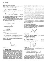
= 2l+1. The degeneracy is lifted by the Zeeman-splitting
degenerate, Σm
l =−l
which is linear in Bml (Fig. 1.4). In the case of strictly vanishing quantum
defects (1.37), different l-values become also degenerate, which may lead to
the more complicated “quadratic Zeeman effect”.
Whereas p2 = −¯h2 ∇2 is a real operator with real eigenfunctions (remember (1.28)), π 2 is complex and does require complex eigenfunctions. A real
eigenfunction can only depend on m2l , not on ml . The Zeeman shift demonstrates the necessity of complex functions. The eigenvalues E remain real,
due to the hermiticity of operators, see Sect. 1.8.

1.5 Bound States
Conducting electrons in metals move like free particles in a constant potential
of depth −V0 , which is measured from the ionization limit to the bottom of
the conducting band. Due to the Pauli principle, they fill all levels of energies
E < EF , where EF < 0 is the Fermi energy. It is customary here to shift
the energy scale such that one has V = 0 inside the metal. The asymptotic
region where (1.75) applies, (k2 + ∇2 )ψ = 0, is then inside the metal. The
details of the metal surface are often unimportant, and it is convenient to
use the limit V = +V0 → ∞ there. In this limit, ψ must vanish at the

www.pdfgrip.com


1.5 Bound States

17

surface, precisely as the standing waves in the waveguide mentioned near the
end of Sect. 1.1. Consider now a wire along the z-axis, with a rectangular
basis of dimensions Lx , Ly . The appropriate solutions of the wave equation
are
ψ(x, y, z) = eikz z sin kx x sin ky y,

sin ki Li = 0 (i = 1, 2).

(1.93)

The last two conditions imply
ki = ni π/Li ,

ni = 1, 2, 3, 4, 5, . . .

(1.94)

whereas kz remains arbitrary, positive or negative. If one now cuts the
wire at zmax = Lz , kz must also be positive and obey condition (1.94)
for i = 3. The possible energy levels are then suddenly discrete or “quantized”,
m2 c4 + c2 ¯h2 k2 =

m2 c4 + c2 (n2x /L2x + n2y /L2y + n2z /L2z )h2 /4,
(1.95)
with h
¯ π = h/2. For a macroscopic piece of metal, one hastens to the limit
Lx = Ly = Lz → ∞, where the energy levels become again dense within
the conducting band (thence the name “band”). Our point here is the opposite one, namely confining the wavefunction to a finite volume Lx Ly Lz
entails a discrete energy spectrum. This is the massive particle analogue of
a microwave cavity, where the modes are quantized according to

E=

¯ ω = (n2x /L2x + n2y /L2y + n2z /L2z )1/2 ch/2.
E(nx , ny , nz ) = h

(1.96)

But whereas a single cavity mode can host many photons, a mode in a metal
can host at most two electrons, due to the Pauli principle (the factor 2 accounts for the electron spin). The modes for electrons are commonly called
“orbitals”. Such modes exist approximately also in a single many-electron
atom. In the simplest form of the atomic shell model, the orbitals are successively filled with electrons. The word “state”, on the other hand, means
a precise wave function. In single-particle problems, there is hardly any difference. But the ground state of the helium atom has a wave function ψ(r1 , r 2 ),
which depends on the two electon positions r1 and r2 . It is an antisymmetrized product of orbitals only if the mutual repulsion of the two electrons
is either neglected or approximated by an over-all weakening of binding. In
the mathematical sense, the concept of a “state” is more general than a wave
function, as will be explained in Sect. 1.9.
The wavefunction of a single spinless particle can be bound by an attractive, spherically symmetric potential V (r) < 0, r = (x2 + y 2 + z 2 )1/2
according to (1.76), but now with A = 0, π 2 = p2 = −¯h2 ∇2 . In spherical
coordinates (1.6), (1.22), ψ(r) has solutions that factorize into angular and
radial parts,
ψk2 (r) = Ylml (θ, φ)Rk2 ,l (r).
(1.97)

www.pdfgrip.com