Tài liệu Báo cáo khoa học: "Bridging the Gap Between Underspecification Formalisms: Hole Semantics as Dominance Constraints" ppt
Bạn đang xem bản rút gọn của tài liệu. Xem và tải ngay bản đầy đủ của tài liệu tại đây (443.97 KB, 8 trang )
Bridging the Gap Between Underspecification Formalisms:
Hole Semantics as Dominance Constraints
Alexander Koller
Joachim Niehren
Stefan Thater
-
sb.de
-
sb.de
-
sb.de
Saarland University, Saarbriicken, Germany
Abstract
We define a back-and-forth translation
between Hole Semantics and dominance
constraints, two formalisms used in un-
derspecified semantics. There are funda-
mental differences between the two, but
we show that they disappear on practi-
cally useful descriptions. Our encoding
bridges a gap between two underspeci-
fication formalisms, and speeds up the
processing of Hole Semantics.
1 Introduction
In the past few years there has been consider-
able activity in the development of formalisms for
underspecified semantics (Alshawi and Crouch,
1992; Reyle, 1993; Bos, 1996; Copestake et al.,
1999; Egg et al., 2001). These approaches all aim
at controlling the combinatorial explosion of read-
ings of sentences with multiple ambiguities. The
common idea is to delay the enumeration of all
readings for as long as possible. Instead, they work
with a compact
underspecified representation
for
as long as possible, only enumerating readings
from this representation by need.
At first glance, many of these formalisms seem
to be very similar to each other. Now the ques-
tion arises how deep this similarity is — are all
underspecification formalisms basically the same?
This paper answers this question for Hole Se-
mantics and normal dominance constraints, two
logical formalisms used in scope underspecifica-
tion, by defining a back-and-forth translation be-
tween the two. Due to fundamental differences
in the way the two formalisms interpret under-
specified descriptions, this encoding is only cor-
rect in a nonstandard sense. However, we identify
a class of
chain-connected
underspecified repre-
sentations for which these differences disappear,
and the encoding becomes correct. We conjecture
that all linguistically useful descriptions are chain-
connected. To support this claim, we prove that all
descriptions generated by a nontrivial grammar we
define are indeed chain-connected.
Our results are interesting because it is the first
time in the literature that two practically relevant
underspecification formalisms are formally related
to each other. In addition, the satisfi ability prob-
lems of Hole Semantics and normal dominance
constraints coincide on their chain-connected frag-
ments. This means that satisfiability of Hole Se-
mantics, which is NP-complete in general (Al-
thaus et al., 2003), becomes polynomial in prac-
tice, and can be checked using the efficient algo-
rithms available for normal dominance constraints
(Erk et al., 2002). Enumeration of readings be-
comes much more efficient accordingly.
2 Some Intuitions
The similarity of Hole Semantics and dominance
constraints is illustrated in Fig. 1. The pictures
graphically represent the underspecified represen-
tations of all five readings of the sentence "Every
researcher of a company saw a sample" in Hole
Semantics (Bos, 1996) and as a dominance con-
straint (Egg et al., 2001). The underspecified rep-
resentations specify the material that every reading
is made up of and constraints on the way in which
they can be combined in obviously similar ways.
However, the interpretations of these under-
specified representations differ. In Hole Seman-
tics, the interpretation is given by means of
plug-
gings, where holes (the
h
i
)
and labels
(/k)
are iden-
tified. In contrast, dominance constraints are inter-
preted by
embedding
descriptions into trees that
may contain more material. This difference comes
195
EA"
comp
>h0<
•
:du.
(comp(u)
A )
12 : Vw.((//2 A
res(w))
h)
:x.(sample(x).4
1/4)
14 : of (w,
u)
15:
see(x,
Figure 1: Graphical representations of the Hole Semantics USR (left) and the normal dominance con-
straint (right) for the sentence "Every researcher of a company saw a sample."
out especially clearly in a description like in Fig. 2.
It has no plugging in Hole Semantics, as two dif-
ferent things would have to be plugged into one
hole, but it is satisfiable as a dominance constraint.
It is this fundamental difference that restricts our
result in §5, and that we avoid by using chain-
connected descriptions.
f
a
b.
4
Figure 2: A description on which Hole Semantics
and dominance constraints disagree.
3
Dominance Constraints
Dominance constraints are a general framework
for the partial description of trees. They have been
used in various areas of computational linguis-
tics (Rogers and Vijay-Shanker, 1994; Gardent
and Webber, 1998). For underspecified semantics,
we consider semantic representations like higher-
order formulas as trees.
Dominance constraints can be extended to
CLLS (Egg et al., 2001), which adds parallelism
constraints to model ellipsis and binding con-
straints to account for variable binding without us-
ing variable names. We do not use these extensions
here, for simplicity, but all results remain true if
we allow binding constraints.
3.1 Syntax and Semantics
We assume a signature E of function symbols
ranged over by
f ,g,
each of which is equipped
with an arity ar(f) > 0, and an infinite set Vars
of variables ranged over by
X,
Y,
Z.
A dominance
constraint c is a conjunction of dominance, in-
equality, and labeling literals of the following
form:
::=
X <
*
Y XY X:f (Xi, • • • ,X01
(
I
)
AC
'
where ar(f) =
n.
Dominance constraints are interpreted over fi-
nite constructor trees, and their variables denote
nodes of a tree. We define an
unlabeled tree
to be a
finite directed acyclic graph (V,
E),
where V is the
set of nodes and ECVxV the set of edges. The
indegree of each node is at most 1. Each tree has
exactly one node (the
root)
with indegree 0. Nodes
with outdegree 0 are called the leaves of the tree.
A finite
constructor tree
T
is a triple
(T,Lv , LE)
consisting of an unlabeled tree
T = (V, E),
a node
labeling
Lv :V —>
E„ and an edge labeling
LE
:
E
N,
s. t. for each node
u E V there is an edge
(u, v)
E
E
with
LE((U,V))
=
k
1 <
k < ar(Lv (u)).
Now we are ready to define tree structures, the
models of dominance constraints:
Definition 1 (Tree Structure). The
tree structure
Mt
of a constructor tree
T =
((V,E),Lv,LE)
is
a first-order structure with domain V interpreting
dominance and labeling.
Let
u,
v, vi, E V. The dominance relation-
ship
u<*
t
v holds if there is a path from
u
to v
in
E
and the labeling relationship
u: ft (vi , ,v„)
holds iff
u
is labeled by the n-ary symbol
f
and
has the children v , , v
n
in this order; that is,
L
v
(u)
=
f,
ar(f) =
n, {(u,v 1), ,(u,v„)} C E,
and
LE((lt,Vi)) = i
for all 1 <
i
<
n.
Let c be a dominance constraint and Var((p) be
the set of variables of c. A pair of a tree structure
glit and a
variable assignment
a: Var((p) 14,
satisfies
( if it satisfies each literal in the obvious
way. We say that (Mt, a) is a
solution
of p in this
case; c is
satisfiable
if it has a solution.
Entailment
c' holds between two constraints if every so-
lution of c is also a solution of
We often represent dominance con-
straints as (directed)
constraint graphs;
for example, the graph in Fig. 2 stands
for the constraint
X
:
f (Y)
A Y
<
*
z
A Y<
*
Z
i
A
Z :a
A
Z' :b.
This constraint is satisfied e.g. by the tree
structure displayed here. Note the added
g.
f
g
a
bo
196
3.2 Solving Dominance Constraints
The satisfiability problem of dominance con-
straints (i.e. deciding whether a constraint has a
solution) is NP-complete (Erk et al., 2002). How-
ever, Althaus et al. (2003) show that satisfiability
becomes polynomial if the constraint (p is normal,
i.e. satisfies the following very natural conditions:
(Ni)
Every variable occurs in a labeling con-
straint.
(N2)
Every variable occurs at most once on the
right-hand side and at most once on the left-
hand side of a labeling constraint. Variables
that don't occur on a left-hand side are called
holes;
variables that don't occur on a right-
hand side are called
roots.
(N3)
If X <1*Y occurs in (p,
X
is a hole and Y is a
root.
(N4)
If
X
and Y are different variables that are not
holes, there is a constraint
X Y
in (p.
The graph of a normal constraint (e.g. the one in
in Fig. 1) consists of solid tree fragments (Ni, N2)
that are connected by dominance edges (N3); these
fragments may not overlap in a solution (N4).
Because every satisfiable dominance constraint
(p has an infinite number of solutions, algorithms
typically enumerate its
solved forms
instead (Erk
et al., 2002). A solved form is a constraint that dif-
fers from (p only in its dominance literals. Its graph
must be a tree, and the reachability relation on the
graph must include the reachability in the graph of
(p. Every solved form of (p has a solution, and every
solution of (p satisfies one of its solved forms; so
we can see solved forms as representing classes of
solutions that only differ in irrelevant details (e.g.
unnecessary extra material).
Another way to avoid infinite solutions sets is
to consider constructive solutions
only. A solution
PI,
a) of a constraint (p is constructive if every
node in
M
is denoted by a variable in Var((p) on
the left-hand side of a labeling constraint. Intu-
itively, this means that the solution consists only of
the material mentioned in the labeling constraints.
Not all solutions are constructive; for example,
Fig. 2 is a solved form but has no constructive so-
lutions. The problem of deciding whether a normal
dominance constraint does have constructive solu-
tions is again NP-complete (Althaus et al., 2003).
4 Hole Semantics
Hole Semantics (Bos, 1996) is a framework that
defines underspecified representations over arbi-
trary object languages. We use the version of
(B Os,
2002) because it repairs some severe flaws in the
original definition of admissible pluggings.
Hole Semantics configures formulas of an ob-
ject language (such as FOL or DRT) with
holes,
into which other formulas can be plugged. For-
mally, a formula with
n
holes is a complex func-
tion symbol of arity
n
as above. The equivalent of
a dominance constraint is an
underspecified repre-
sentations
(USR). An USR
U
consists of a finite
set
L
u
of labeled formulas
1:F (h
i
, ,h
0
),
where
1
is a label and
F
is an object-language formula with
holes
,hn,
and a finite set
C
u
of constraints.
Constraints are of the form
I< h,
where / is a label
and
h a hole; this constraint means that h outscopes
1.
Like for dominance constraints, there is a natural
way of writing USRs as graphs (Fig. 1).
An USR
U
is called
proper
if it has the follow-
ing properties:
(P1)
U
has a unique
top element,
from which all
other nodes in the graph can be reached.
(P2)
The graph of
U
is acyclic.
(P3)
Every label and every hole except for the top
hole occurs exactly once in
Lu .
1
For example, the USR shown in Fig. 1 is proper;
its top element is
11
0
.
The solutions of underspecified representations
are called
admissible pluggings.
A plugging is a
bijection from the holes to the labels of an USR.
Intuitively, we "plug" every hole with a formula
(named by its label), and a plugging is admissible
if it respects the constraints on the order of holes
and labels.
Definition 2 (P-domination).
Let
k, k'
be holes
or labels of some underspecified representation
U,
and
P
a plugging on
U.
Then k P-dominates k'
iff
one of the following conditions holds:
1.
k : F E
Lu
and
k'
occurs in
F,
or
2.
P(k)
I('
if
k
is a hole, or
3. There is a hole or label
k"
such that
k P-
dominates
k"
and
k"
P-dominates
k'.
1
The restriction on hole occurrences is missing in (Bos,
2002), but is necessary to rule out counterintuitive USRs.
197
Definition 3 (Admissible Plugging). A plugging
P
is
admissible
for a proper USR
U
iff
k <
E
Cu
implies that
lc'
P-dominates
k.
5 Hole Semantics as Dominance
Constraints
Now we have the formal machinery to make the
intuitive similarity between Hole Semantics and
dominance constraints described in Section 2 pre-
cise. We shall define encodings from Hole Seman-
tics to normal dominance constraints and back,
and show that this preserves models in a certain
sense.
To keep things simple, the results in this sec-
tions will only speak about compact
normal domi-
nance constraints. A dominance constraint is com-
pact if no variable occurs in two different labeling
constraints. A very nice property (which we need
below) of compact normal constraints is that every
variable is either a root or a hole. However, any
normal constraint can be made compact by an op-
eration called compactification, which compresses
conjunctions of labeling constraints into single la-
beling constraints with more complex labels. So
the encodings and results are more more generally
correct for arbitrary normal dominance constraints
(with acyclic graphs).
From Hole Semantics to Dominance Con-
straints. Assume
U = (L
u
,C
u
)
is a proper USR.
To obtain a compact dominance constraint (p
u
that
encodes the same information, we first encode ev-
ery labeled formula
1:F (hi, ,h)
as the labeling
constraint
1:F (h
i
, ,h,).
We encode every con-
straint / <
h
in
C
u
as a dominance constraint
h<* 1
— except if
h
is the unique top hole and does not
occur as a hole in a labeled formula. Finally, we
add a constraint / 1' for every label
1.
This encoding maps labels and holes to vari-
ables; labels end up as roots, and holes become
holes. This means (p
u
satisfies axiom (N3). (N2)
follows from (P3). (Ni) and (N4) are obvious from
the construction. Hence (p
u
is normal.
From Dominance Constraints to Hole Se-
mantics. Assume (p is a compact normal domi-
nance constraint whose graph is acyclic. To ob-
tain a proper USR U
T
encoding the same infor-
mation, we first split the variables Var((p) into
holes and labels: roots become labels, and holes
become holes. Then we encode every labeling
constraint
X:f(Xi, ,X,
i
)
as the labeled formula
X: f (Xi , ,X,
1
),
and we encode every dominance
constraint
X
<I' as the constraint Y <
X.
Finally,
we add a top hole
ho
and a constraint / < ho for
every label
1
in U.
U
T
is a well-defined USR because of (N3). (P1)
is obvious:
ho
is the unique top element. The graph
is acyclic because the graph of (p is acyclic, so
(P2) holds. (P3) holds because every label names
at least one formula by construction, and no more
than one by (N2).
This back-and-forth encoding has the following
property:
Theorem 4.
Compact normal dominance con-
straints ç with acyclic graphs and proper USRs U
can be encoded into each other, in such a way that
the pluggings of U and the constructive solutions
of
9
correspond.
Proof
We only show that the solutions of an USR
U
and its encoding
cu
correspond; the other direc-
tion is analogous.
Assume first that we have a plugging
P
of
U.
We build a tree which satisfies
cu
constructively
and has one node for every label
1
of
U.
The node
label of this node is the formula that
1
addresses.
Starting at the top element, we work our way down
the USR; whenever we find a hole
h,
we continue
at the label
P(h).
Conversely, assume we have a constructive so-
lution
M
of
9.
Every node in
/I
is denoted by
a variable. Because holes have no labeling con-
straints, every hole
h
must denote the same node
as a root
P(h
). Further, every root that is not the
root of the entire tree denotes the child of another
root, i.e. denotes the same node as a hole. We ob-
tain an admissible plugging by mapping each hole
h
to the label
P(h
) in the USR, and mapping the
new top hole 1/0 to the label denoting the root of
the tree.
6 From Solved Forms to Constructive
Solutions
Theorem 4 establishes a very strong connec-
tion between Hole Semantics and normal dom-
inance constraints. But it is not quite what we
want: Normal dominance constraints are almost
198
always considered with respect to arbitrary solu-
tions (or solved forms), and not constructive solu-
tions. Constraints such as Fig. 2 are solved forms,
but have no constructive solutions. The efficient
algorithms available for normal constraints check
for solved forms, and aren't necessarily correct for
constructive satisfiability.
In this section, we establish that for normal
dominance constraints which are
chain-connected
and
leaf-labeled
(to be defined below), satisfia-
bility and constructive satisfiability are equiva-
lent; i.e. such a constraint has a constructive so-
lution if only it is satisfiable. The proof proceeds
in three steps: First we show that all solved forms
of a normal constraint are
simple
iff the constraint
branches constructively.
Then we show that if
a constraint is chain-connected, it branches con-
structively. Finally, every simple solved form of a
leaf-labeled constraint has a constructive solution.
6.1 Constructive Branching
We call a solved form
simple
if its graph has
no node with two outgoing dominance edges (i.e.
Fig. 2 is
not
simple). This means that we can de-
cide for any two variables how they will be sit-
uated in a solution of the solved form. They can
either dominate each other in either direction, or
they can be
disjoint.
But if they are disjoint, we
also know the lowest node that dominates them
both, and this branching point
is necessarily also
denoted by a variable on the left-hand side of a
labeling constraint.
This motivates the following definition. We lo-
cally allow disjunctions of constraints and use
an auxiliary constraint, the disjointness constraint
X
I Y at
0,
where
0
is a set of variables. It is
satisfied if
X
and Y denote disjoint nodes whose
branching point is denoted by a member of
0.
Definition 5.
A normal dominance constraint (p
branches constructively
if for any two variables
X ,Y E Var((p),
X<*Y V
Y<*X
V
X
_L Y at L((p),
where L((p) is the set of variables that occur on the
left-hand side of a labeling constraint in (p.
Lemma 6. Let
(p
be a normal dominance con-
straint.
(p
branches constructively if all solved
forms of
y
are simple.
Proof
Assume first that all solved forms of (p are
simple; let
{(pi,
, (pd- be the set of all solved
forms. Now because they are simple solved forms,
each (p
i
entails the right-hand side of Def. 5. But
(p entails the disjunction of all of its solved forms,
and hence branches constructively.
Conversely, assume that (p has a non-simple
solved form (V. Then (p' must contain a variable
X
with two outgoing dominance edges (to Y and
Z).
But this means that (p' has a solution in which
Y and Z are different children of
X,
and hence their
lowest common ancestor is not in L((p).
6.2 Chain-Connectedness
Constructive branching is a semantic property that
can't conveniently be proved for a grammar. We
shall now relate it to a more easily checkable prop-
erty called
chain-connectedness.
We will first de-
fine chains, then chain-connectedness, and then
prove the relation of the two concepts.
Definition 7 (Fragments).
A
fragment
in (p is a
nonempty subset
F
C Va r((p) that is connected
by labeling constraints in (p. We call the fragment
maximal
if it has no proper superset that is also a
fragment of (p. Exactly one variable in every frag-
ment is a root; we write
R(F)
for this root.
Definition 8 (Chains).
Let (p be a normal domi-
nance constraint, and let
F
1
, , F
n
(n > 1)
be dis-
joint fragments of (p.
C = (F1, ,F)
is called a
chain
of (p iff there is a disjoint partition
0
U U =
{F1 , , F„} with the following properties:
1.
0
is nonempty.
2.
For each 1 < <
n,
either
(a)
Fi
E
0
and F
t+
i
E
U, and there is a hole
of
F
i
s.t.
Xj,,,:i*R(Fi+i);
or
(b)
F,
E U
and F
i+
E
0,
and there is a hole
X
i+
1,1
of
Ji
s.t.
X,+1,/<*R(Fi).
3. For 1 <
i
<
n s.t. F
i
E
0,
the holes
X
1
,1
and
are different.
0
is called the set of
upper fragments
of the chain,
and
QI
is the set of
lower fragments.
We call all the
X
j
,1
and Xi
,
r
connecting holes
of
C,
and all other
holes in any of its fragments
open holes.
A schematic picture of a chain is shown in
Fig. 3. Note that although the definition of a chain
involves the rather abstract condition that domi-
nance between to variables is entailed by the con-
199
Figure 3: A schematic picture of a chain.
straint, this condition can often be established syn-
tactically — for example in Fig. 3 by the explicit
dominance edges. Chains were originally intro-
duced by Koller et al. (2000) because they have
very useful structural properties. A particularly
useful one is the following.
Lemma 9 (Structural Properties of Chains).
Let
(p
be a normal dominance constraint, and let C be
a chain that contains all variables of
(p.
Let
be the set of all variables in upper fragments of
C that are not holes. Then if X,Y are variables in
different fragments of C, the following structural
property holds:
X <*Y V Y
<*X
V
X
I Y at
`120
Using this lemma, it is easy to show that
whenever a constraint is chain-connected, it also
branches constructively.
Definition 10. Two variables
X,
Y of a normal
dominance constraint (p are
chain-connected in
(p
if there is a chain
C
in ç that contains both
X
and
Y. A constraint is
chain-connected
iff every pair of
variables is chain-connected.
Proposition 11.
Every chain-connected domi-
nance constraint
(p
branches constructively.
Proof
Let
X,
Y be two arbitrary variables in (p.
If
X
and Y belong to the same fragment, there is
obviously a connecting chain containing just this
fragment. Otherwise, constructive branching for
X
and Y follows from Lemma 9.
For the last step of the proof, we define that a
normal dominance constraint is
leaf-labeled
if ev-
ery variable occurs on the left-hand side of a label-
ing or dominance literal. Such constraints have the
following property:
Lemma 12.
Every simple solved form of a leaf-
labeled constraint has a constructive solution.
Putting it all together, we obtain the intended
result:
Theorem 13.
Every solved form of a chain-
connected, leaf-labeled normal dominance con-
straint has a constructive solution.
We can transfer the notions of chain-
connectedness and leaf-labeledness to USRs
either by a direct definition or by defining that
U
is chain-connected or leaf-labeled iff y
u
is. Then
we can state the following theorem:
Corollary 14 (Processing of Hole Semantics).
The problem whether a chain-connected, leaf-
labeled proper USR has a plugging is polynomial.
Proof
Simply check the corresponding dom-
inance constraint for satisfiability. Althaus
et al. (2003) give a quadratic satisfiability algo-
rithm; Thiel (2002) improves this to linear.
7 Connectedness in a Grammar
Finally, we claim that chain-connectedness and
leaf-labeledness are very weak assumptions to
make about a normal dominance constraint, and
conjecture that all linguistically useful constraints
satisfy them. We define a nontrivial grammar for
a fragment of English and show that it only gen-
erates dominance constraints with these proper-
ties. The argument we use to establish chain-
connectedness (the less obvious property) is fairly
general, and should be applicable to other gram-
mar fragments as well.
The grammar we use is a variant of the one pre-
sented in (Egg et al., 2001). Its syntax-semantics
interface produces dominance constraints describ-
ing formulas of higher-order logic; the symbol @
stands for functional application, and abstraction
and variables are written as 'lam,' and `var
x
'. We
use dominance constraints because this gives us
the logical tools we need in the proof; but by
Theorem 4, we can translate all results back into
proper USRs, and those USRs will also be chain-
connected.
7.1 The Grammar
The syntactic component of the grammar consists
of the following phrase structure rules.
200
•
[v:Np Det N] V
(b9)
[v:N
N
]
Var
x
(bit)
[v:Rc RPi S]
[
vs]
N RC]
(
T
)
Varx
Xvr„ •
var
y
e
X,;"
var
y
w
e
x; where (W, a)
E
Lex
(b I)
(b2)
(b3)
(b4)
(b5)
(b7)
[vs
NP VP]
[v:vp IV]
[v:vp TV NP]
[v:vp RV NP VP]
[v:vp SV S]
[v:Np PN]
v'
@
'"
v'e•
X
v
r„
vf"
@
^C
x
v
r„
var
x
e; )q
.
,`
Figure 4: The syntax-semantics interface
(al) S
NP VP
(a8) NP Det N
(a2)
VP —*IV
(a9) N N
(a3)
VP TV NP
(a10) N —*N RC
(a4)
VP RV NP VP (all) RC —> RP S
(a5)
VP
SV S
(a13)
W
(a7) NP
PN
if (W, oc)
E
Lex
Most category labels are self-explanatory, perhaps
except for SV, which refers to verbs taking sen-
tence complements such as
say,
and RV, which
refers to (object) raising verbs such as
expect.
The lexicon is defined by a relation
Lex
relating
words and lexical categories. Rule (al 3) expands
lexical categories to words of the category.
7.2 The Syntax-Semantics Interface
Every node v in a syntax tree contributes a con-
straint (p
v
; the variable X is intuitively the "root"
of this contribution. We assume that the syntax
provides for a coindexation of relative pronouns
and their corresponding traces, and associate each
NP with index
i
with a corresponding variable
X.
The variables are related by the rules in Fig. 4.
Each syntactic production rule corresponds to one
semantic construction rule, which defines the se-
mantic contribution of a syntactic node. A con-
struction rule of the form
[
vy
Q Tv
means
that the node v in the syntax tree is labeled with P,
and its two daughter nodes
v
1
and
v"
are labeled
with
Q
and R,
respectively. The semantic contribu-
tion of v is the constraint (pv , with fresh instances
of 'lam,' and 'var
.
,' where necessary.
The complete constraint of a syntax tree with
root v is the conjunction of the (pv for all nodes
v'
dominated by v, and inequalities that are needed
to make the constraint norma1.
2
7.3 Connectedness of Constraints
The proof that all constraints generated by this
grammar are connected proceeds by structural in-
duction over parse trees. The semantic contribu-
tions of leaves are trivially chains, and hence con-
nected. What we show in the rest of this section is
that if
t
is any subtree of the syntax tree, and all the
semantics of all immediate subtrees of
t
are con-
nected, then so is the semantics of
t.
We ignore the
globally introduced inequality constraints because
they have no effect on chain-connectedness.
The central property of the construction rules
that we exploit is the following:
Proposition 15.
Let
Po, (p,
be chain-
connected constraints such that
1.
Var((p
i
)
n
Var((p
j
) = 0,
for 1 < i < j n,
2.
Var((p
o
)
n
Var( (p
i
) = {X
i
},
for 1 <i < n,
where
,Xn are open holes in all connecting
chains in
y
o
.
Then the constraint
y
o
A • A (p
0
is
chain-connected.
2
The original grammar accounts for scope island con-
straints by means of additional dominance literals. We ignore
them here, as they do not affect chain-connectedness.
201
This can be proved by induction. The base case
n = 0
is trivial, and for the induction step we
combine a connecting chain within (p
0
A • • • A
(p„_
1
from an arbitrary
X
to
X,
with a connecting chain
within (p„ from
X,
to an arbitrary Y. Chains are
combined by taking all the fragments of the two
smaller chains together. The assumption that the
Xi
are open holes in the connecting chains is needed
for the problematic case in which the fragment
containing
X,
is an upper fragment in both chains.
All constraints introduced by a semantics con-
struction rule other than (b11) are of this form:
(p
0
corresponds to the constraint introduced by
the rule, and (p1, , (p
n
to the constraints asso-
ciated with the daughter nodes. Hence, all con-
straints generated using only these rules are chain-
connected. For the case of (b11), observe that the
relative pronoun is coindexed with its trace. This
means that the variable
X
‘
C,
occurs in the same frag-
ment as so (b11) also satisfies the general
scheme. An easier structural induction shows that
the constraints are also leaf-labeled. Hence:
Corollary 16.
All constraints generated by the
grammar are chain-connected and leaf-labeled.
8 Conclusion
We have established the equivalence of Hole Se-
mantics and normal acyclic dominance constraints
with constructive solutions. They are equivalent
to normal acyclic dominance constraints with
standard solutions if the constraints are chain-
connected and leaf-labeled. All constraints gen-
erated by our grammar have these properties; we
conjecture this is true more generally.
This bridges a gap between the two underspeci-
fication formalisms, which means that we can now
combine the simplicity of hole semantics with the
efficient algorithms, powerful metatheory, and ex-
tensibility of dominance constraints. A first prac-
tically useful result is a polynomial satisfiability
algorithm for chain-connected, leaf-labeled USRs.
Conversely, chain-connected dominance con-
straints inherit some of Hole Semantics' resource-
sensitivity: Additional material
need
never be
added to satisfy the constraint; but to model e.g.
reinterpretation (Koller et al., 2000), this is still
possible. This resource-sensitivity was the crucial
difference between the two formalisms. In the fu-
ture, it will be interesting to see how our results
extend to other resource-sensitive underspecifica-
tion formalisms — for example, to MRS (Copes-
take et al., 1999), whose naive encoding into dom-
inance constraints is less obviously normal, and
which adds a more powerful outscopes relation.
References
H.
Alshawi and R. Crouch.
1992.
Monotonic semantic
interpretation. In
Proc. 30th ACL,
pages 32-39.
E. Althaus, D. Duchier, A. Koller, K. Mehlhorn,
J. Niehren, and S. Thiel. 2003. An effi cient graph
algorithm for dominance constraints.
Journal of Al-
gorithms.
In press.
Johan Bos. 1996. Predicate logic unplugged. In
Proc.
10th Amsterdam Colloquium,
pages 133-143.
J.
Bos. 2002.
Underspecifi
cation and resolution in dis-
course semantics.
Ph.D. thesis, Saarland University.
A. Copestake, D. Flickinger, and I. Sag. 1999. Mini-
mal Recursion Semantics. An Introduction. Unpub-
lished manuscript.
M. Egg, A. Koller, and J. Niehren. 2001. The con-
straint language for lambda structures.
Journal of
Logic, Language, and Information,
10:457-485.
K.
Erk, A. Koller, and J. Niehren. 2002. Processing
underspecifi ed semantic representations in the con-
straint language for lambda structures.
Research in
Language and Computation, 1(1).
In Press.
Claire Gardent and Bonnie Webber. 1998. Describ-
ing discourse semantics. In
Proceedings of the 4th
TAG+ Workshop,
Philadelphia.
A. Koller, J. Niehren, and K. Striegnitz. 2000. Relax-
ing underspecifi ed semantic representations for rein-
terpretation.
Grammars,
3(2-3).
Uwe Reyle. 1993. Dealing with ambiguities by under-
specifi cation: construction, representation, and de-
duction.
Journal of Semantics, 10:123-179.
J. Rogers and K. Vijay-Shanker. 1994. Obtaining
trees from their descriptions: An application to tree-
adjoining grammars.
Computational Intelligence,
10:401-421.
Sven Thiel. 2002. A linear time algorithm for the con-
fi guration problem of dominance graphs. Submit-
ted.
202