Tài liệu Báo cáo khoa học: "Selecting the “Right” Number of Senses Based on Clustering Criterion Functions" pdf
Bạn đang xem bản rút gọn của tài liệu. Xem và tải ngay bản đầy đủ của tài liệu tại đây (93.13 KB, 4 trang )
Selecting the “Right” Number of Senses
Based on Clustering Criterion Functions
Ted Pedersen and Anagha Kulkarni
Department of Computer Science
University of Minnesota, Duluth
Duluth, MN 55812 USA
{tpederse,kulka020}@d.umn.edu
Abstract
This paper describes an unsupervised
knowledge–lean methodology for auto-
matically determining the number of
senses in which an ambiguous word is
used in a large corpus. It is based on the
use of global criterion functions that assess
the quality of a clustering solution.
1 Introduction
The goal of word sense discrimination is to cluster
the occurrences of a word in context based on its
underlying meaning. This is often approached as a
problem in unsupervised learning, where the only
information available is a large corpus of text (e.g.,
(Pedersen and Bruce, 1997), (Sch
¨
utze, 1998), (Pu-
randare and Pedersen, 2004)). These methods usu-
ally require that the number of clusters to be dis-
covered (k) be specified ahead of time. However,
in most realistic settings, the value of k is unknown
to the user.
Word sense discrimination seeks to cluster N
contexts, each of which contain a particular tar-
get word, into k clusters, where we would like
the value of k to be automatically selected. Each
context consists of approximately a paragraph of
surrounding text, where the word to be discrimi-
nated (the target word) is found approximately in
the middle of the context. We present a methodol-
ogy that automatically selects an appropriate value
for k. Our strategy is to perform clustering for suc-
cessive values of k, and evaluate the resulting solu-
tions with a criterion function. We select the value
of k that is immediately prior to the point at which
clustering does not improve significantly.
Clustering methods are typically either parti-
tional or agglomerative. The main difference is
that agglomerative methods start with 1 or N clus-
ters and then iteratively arrive at a pre–specified
number (k) of clusters, while partitional methods
start by randomly dividing the contexts into k clus-
ters and then iteratively rearranging the members
of the k clusters until the selected criterion func-
tion is maximized. In this work we have used K-
means clustering, which is a partitional method,
and the H2 criterion function, which is the ratio
of within cluster similarity to between cluster sim-
ilarity. However, our approach can be used with
any clustering algorithm and global criterion func-
tion, meaning that the criterion function should ar-
rive at a single value that assesses the quality of the
clustering for each value of k under consideration.
2 Methodology
In word sense discrimination, the number of con-
texts (N ) to cluster is usually very large, and con-
sidering all possible values of k from 1 N would
be inefficient. As the value of k increases, the cri-
terion function will reach a plateau, indicating that
dividing the contexts into more and more clusters
does not improve the quality of the solution. Thus,
we identify an upper bound to k that we refer to as
deltaK by finding the point at which the criterion
function only changes to a small degree as k in-
creases.
According to the H 2 criterion function, the
higher its ratio of within cluster similarity to be-
tween cluster similarity, the better the clustering.
A large value indicates that the clusters have high
internal similarity, and are clearly separated from
each other. Intuitively then, one solution to select-
ing k might be to examine the trend of H 2 scores,
and look for the smallest k that results in a nearly
maximum H2 value.
However, a graph of H 2 values for a clustering
111
of the 4 sense verb serve as shown in Figure 1 (top)
reveals the difficulties of such an approach. There
is a gradual curve in this graph and the maximum
value (plateau) is not reached until k values greater
than 100.
We have developed three methods that take as
input the H 2 values generated from 1 deltaK
and automatically determine the “right” value of
k, based on finding when the changes in H 2 as k
increases are no longer significant.
2.1 PK1
The P K1 measure is based on (Mojena, 1977),
which finds clustering solutions for all values of
k from 1 N , and then determines the mean and
standard deviation of the criterion function. Then,
a score is computed for each value of k by sub-
tracting the mean from the criterion function, and
dividing by the standard deviation. We adapt this
technique by using the H2 criterion function, and
limit k from 1 deltaK:
P K1(k) =
H2(k) − mean(H2[1 deltaK])
std(H2[1 deltaK])
(1)
To select a value of k, a threshold must be set.
Then, as soon as P K1(k) exceeds this threshold,
k-1 is selected as the appropriate number of clus-
ters. We have considered setting this threshold us-
ing the normal distribution based on interpreting
P K1 as a z-score, although Mojena makes it clear
that he views this method as an “operational rule”
that is not based on any distributional assumptions.
He suggests values of 2.75 to 3.50, but also states
they would need to be adjusted for different data
sets. We have arrived at an empirically determined
value of -0.70, which coincides with the point in
the standard normal distribution where 75% of the
probability mass is associated with values greater
than this.
We observe that the distribution of P K1 scores
tends to change with different data sets, making it
hard to apply a single threshold. The graph of the
P K1 scores shown in Figure 1 illustrates the dif-
ficulty - the slope of these scores is nearly linear,
and as such the threshold (as shown by the hori-
zontal line) is a somewhat arbitrary cutoff.
2.2 PK2
P K2 is similar to (Hartigan, 1975), in that both
take the ratio of a criterion function at k and k-1,
0.001
0.002
0.003
0.004
0.005
0.006
0.007
0.008
0.009
0 50 100 150 200
H2 vs k
s
r
-2.000
-1.500
-1.000
-0.500
0.000
0.500
1.000
1.500
2 3 4 5 6 7 8 9 10 11 12 13 14 15 16 17
PK1 vs k
r
r
r
r
r
r
r
r
r
r
r
r
r
r
r
r
✷
0.900
1.000
1.100
1.200
1.300
1.400
1.500
1.600
1.700
1.800
1.900
2 3 4 5 6 7 8 9 10 11 12 13 14 15 16 17
PK2 vs k
r
r
r
r
r
r
r
r
r
r
r
r
r
r r
r
✷
0.990
0.995
1.000
1.005
1.010
1.015
1.020
1.025
1.030
1.035
1.040
2 3 4 5 6 7 8 9 10 11 12 13 14 15 16 17
PK3 vs k
r
r
r
r
r
r
r
r
r
r
r
r
r
r
r
✷
Figure 1: Graphs of H2 (top) and PK 1-3 for
serve: Actual number of senses (4) shown as trian-
gle (all), predicted number as square (PK1-3), and
deltaK (17) shown as dot (H2) and upper limit of
k (PK1-3).
112
in order to assess the relative improvement when
increasing the number of clusters.
P K2(k) =
H2(k)
H2(k − 1)
(2)
When this ratio approaches 1, the clustering has
reached a plateau, and increasing k will have no
benefit. If P K2 is greater than 1, then an addi-
tional cluster improves the solution and we should
increase k. We compute the standard deviation of
P K2 and use that to establish a boundary as to
what it means to be “close enough” to 1 to consider
that we have reached a plateau. Thus, P K2 will
select k where P K 2(k) is the closest to (but not
less than) 1 + standard deviation(PK2[1 deltaK]).
The graph of P K2 in Figure 1 shows an el-
bow that is near the actual number of senses. The
critical region defined by the standard deviation is
shaded, and note that P K2 selected the value of
k that was outside of (but closest to) that region.
This is interpreted as being the last value of k that
resulted in a significant improvement in cluster-
ing quality. Note that here P K2 predicts 3 senses
(square) while in fact there are 4 actual senses (tri-
angle). It is significant that the graph of P K2 pro-
vides a clearer representation of the plateau than
does that of H2.
2.3 PK3
P K3 utilizes three k values, in an attempt to find
a point at which the criterion function increases
and then suddenly decreases. Thus, for a given
value of k we compare its criterion function to the
preceding and following value of k:
P K3(k) =
2 × H 2(k)
H2(k − 1) + H 2(k + 1)
(3)
P K3 is close to 1 if the three H2 values form
a line, meaning that they are either ascending, or
they are on the plateau. However, our use of
deltaK eliminates the plateau, so in our case values
of 1 show that k is resulting in consistent improve-
ments to clustering quality, and that we should
continue. When P K3 rises significantly above 1,
we know that k+1 is not climbing as quickly, and
we have reached a point where additional clus-
tering may not be helpful. To select k we chose
the largest value of P K3(k) that is closest to (but
still greater than) the critical region defined by the
standard deviation of P K3. This is the last point
where a significant increase in H2 was observed.
Note that the graph of P K3 in Figure 1 shows the
value of P K3 rising and falling dramatically in
the critical region, suggesting a need for additional
points to make it less localized.
P K3 is similar in spirit to (Salvador and Chan,
2004), which introduces the L measure. This tries
to find the point of maximum curvature in the cri-
terion function graph, by fitting a pair of lines to
the curve (where the intersection of these lines rep-
resents the selected k).
3 Experimental Results
We conducted experiments with words that have 2,
3, 4, and 6 actual senses. We used three words that
had been manually sense tagged, including the 3
sense adjective hard, the 4 sense verb serve, and
the 6 sense noun line. We also created 19 name
conflations where sets of 2, 3, 4, and 6 names of
persons, places, or organizations that are included
in the English GigaWord corpus (and that are typ-
ically unambiguous) are replaced with a single
name to create pseudo or false ambiguities. For
example, we replaced all mentions of Bill Clinton
and Tony Blair with a single name that can refer
to either of them. In general the names we used
in these sets are fairly well known and occur hun-
dreds or even thousands of times.
We clustered each word or name using four dif-
ferent configurations of our clustering approach,
in order to determine how consistent the selected
value of k is in the face of changing feature sets
and context representations. The four configura-
tions are first order feature vectors made up of un-
igrams that occurred 5 or more times, with and
without singular value decomposition, and then
second order feature vectors based on bigrams that
occurred 5 or more times and had a log–likelihood
score of 3.841 or greater, with and without sin-
gular value decomposition. Details on these ap-
proaches can be found in (Purandare and Peder-
sen, 2004).
Thus, in total there are 22 words to be discrim-
inated, 7 with 2 senses, 6 words with 3 senses, 6
with 4 senses, and 3 words with 6 senses. Four
different configurations of clustering are run for
each word, leading to a total of 88 experiments.
The results are shown in Tables 1, 2, and 3. In
these tables, the actual numbers of senses are in
the columns, and the predicted number of senses
are in the rows.
We see that the predicted value of P K1 agreed
113
Table 1: k Predicted by PK1 vs Actual k
2 3 4 6
1 6 6 3 3 18
2
5 5 1 3 14
3 4 1 7 2 14
4
6 5 7 1 19
5 4 2 1 7
6
2 3 3 2 10
7 1 1 2
8
1 1
9 1 1 2
11
1 1
28 24 24 12 88
Table 2: k Predicted by PK2 vs Actual k
2 3 4 6
1 3 1 4
2
8 5 7 6 26
3 8 10 8 2 30
4
4 2 3 9
5 1 3 2 6
6
1 2 1 4
7 2 2
9 1 1 2
10
1 2 3
11 1 1
12
1 1
17 2 2
28 24 24 12 88
with the actual value in 15 cases, whereas P K 3
agreed in 17 cases, and P K2 agreed in 22 cases.
We observe that P K1 and P K3 also experienced
considerable confusion, in that their predictions
were in many cases several clusters off of the cor-
rect value. While P K2 made various mistakes,
it was generally closer to the correct values, and
had fewer spurious responses (very large or very
small predictions). We note that the distribution
of P K2’s predictions were most like those of the
actual senses.
4 Conclusions
This paper shows how to use clustering criterion
functions as a means of automatically selecting the
number of senses k in an ambiguous word. We
have found that P K 2, a ratio of the criterion func-
tions for the current and previous value of k, is
Table 3: k Predicted by PK3 vs Actual k
2 3 4 6
1 3 4 1 1 9
2
13 9 12 4 38
3 4 3 4 4 15
4
2 2 1 1 6
5 2 1 1 1 5
6
1 2 3 6
7 1 1 1 3
9
1 1
10 1 1
11
2 2
12
1 1
13
1 1
28 24 24 12 88
most effective, although there are many opportu-
nities for future improvements to these techniques.
5 Acknowledgments
This research is supported by a National Science
Foundation Faculty Early CAREER Development
Award (#0092784). All of the experiments in
this paper were carried out with the SenseClusters
package, which is freely available from the URL
on the title page.
References
J. Hartigan. 1975. Clustering Algorithms. Wiley, New
York.
R. Mojena. 1977. Hierarchical grouping methods and
stopping rules: An evaluation. The Computer Jour-
nal, 20(4):359–363.
T. Pedersen and R. Bruce. 1997. Distinguishing word
senses in untagged text. In Proceedings of the Sec-
ond Conference on Empirical Methods in Natural
Language Processing, pages 197–207, Providence,
RI, August.
A. Purandare and T. Pedersen. 2004. Word sense dis-
crimination by clustering contexts in vector and sim-
ilarity spaces. In Proceedings of the Conference on
Computational Natural Language Learning, pages
41–48, Boston, MA.
S. Salvador and P. Chan. 2004. Determining the
number of clusters/segments in hierarchical cluster-
ing/segmentation algorithms. In Proceedings of the
16th IEEE International Conference on Tools with
AI, pages 576–584.
H. Sch
¨
utze. 1998. Automatic word sense discrimina-
tion. Computational Linguistics, 24(1):97–123.
114