Tài liệu Báo cáo khoa học: "Bayesian Word Sense Induction" pdf

Proceedings of the 12th Conference of the European Chapter of the ACL, pages 103–111,
Athens, Greece, 30 March – 3 April 2009.
c
2009 Association for Computational Linguistics
Bayesian Word Sense Induction
Samuel Brody
Dept. of Biomedical Informatics
Columbia University

Mirella Lapata
School of Informatics
University of Edinburgh

Abstract
Sense induction seeks to automatically
identify word senses directly from a cor-
pus. A key assumption underlying pre-
vious work is that the context surround-
ing an ambiguous word is indicative of
its meaning. Sense induction is thus typ-
ically viewed as an unsupervised cluster-
ing problem where the aim is to partition
a word’s contexts into different classes,
each representing a word sense. Our work
places sense induction in a Bayesian con-
text by modeling the contexts of the am-
biguous word as samples from a multi-
nomial distribution over senses which
are in turn characterized as distributions
over words. The Bayesian framework pro-
vides a principled way to incorporate a

wide range of features beyond lexical co-
occurrences and to systematically assess
their utility on the sense induction task.
The proposed approach yields improve-
ments over state-of-the-art systems on a
benchmark dataset.
1 Introduction
Sense induction is the task of discovering automat-
ically all possible senses of an ambiguous word. It
is related to, but distinct from, word sense disam-
biguation (WSD) where the senses are assumed to
be known and the aim is to identify the intended
meaning of the ambiguous word in context.
Although the bulk of previous work has been
devoted to the disambiguation problem
1
, there are
good reasons to believe that sense induction may
be able to overcome some of the issues associ-
ated with WSD. Since most disambiguation meth-
ods assign senses according to, and with the aid
1
Approaches to WSD are too numerous to list; We refer
the interested reader to Agirre et al. (2007) for an overview
of the state of the art.
of, dictionaries or other lexical resources, it is dif-
ficult to adapt them to new domains or to lan-
guages where such resources are scarce. A re-
lated problem concerns the granularity of the sense
distinctions which is fixed, and may not be en-

tirely suitable for different applications. In con-
trast, when sense distinctions are inferred directly
from the data, they are more likely to represent
the task and domain at hand. There is little risk
that an important sense will be left out, or that ir-
relevant senses will influence the results. Further-
more, recent work in machine translation (Vickrey
et al., 2005) and information retrieval (V
´
eronis,
2004) indicates that induced senses can lead to im-
proved performance in areas where methods based
on a fixed sense inventory have previously failed
(Carpuat and Wu, 2005; Voorhees, 1993).
Sense induction is typically treated as an un-
supervised clustering problem. The input to the
clustering algorithm are instances of the ambigu-
ous word with their accompanying contexts (rep-
resented by co-occurrence vectors) and the output
is a grouping of these instances into classes cor-
responding to the induced senses. In other words,
contexts that are grouped together in the same
class represent a specific word sense. In this paper
we adopt a novel Bayesian approach and formalize
the induction problem in a generative model. For
each ambiguous word we first draw a distribution
over senses, and then generate context words ac-
cording to this distribution. It is thus assumed that
different senses will correspond to distinct lexical
distributions. In this framework, sense distinctions

arise naturally through the generative process: our
model postulates that the observed data (word con-
texts) are explicitly intended to communicate a la-
tent structure (their meaning).
Our work is related to Latent Dirichlet Allo-
cation (LDA, Blei et al. 2003), a probabilistic
model of text generation. LDA models each doc-
ument using a mixture over K topics, which are
in turn characterized as distributions over words.
103
The words in the document are generated by re-
peatedly sampling a topic according to the topic
distribution, and selecting a word given the chosen
topic. Whereas LDA generates words from global
topics corresponding to the whole document, our
model generates words from local topics chosen
based on a context window around the ambiguous
word. Document-level topics resemble general do-
main labels (e.g., finance, education) and cannot
faithfully model more fine-grained meaning dis-
tinctions. In our work, therefore, we create an in-
dividual model for every (ambiguous) word rather
than a global model for an entire document col-
lection. We also show how multiple information
sources can be straightforwardly integrated with-
out changing the underlying probabilistic model.
For instance, besides lexical information we may
want to consider parts of speech or dependen-
cies in our sense induction problem. This is in
marked contrast with previous LDA-based mod-

els which mostly take only word-based informa-
tion into account. We evaluate our model on a
recently released benchmark dataset (Agirre and
Soroa, 2007) and demonstrate improvements over
the state-of-the-art.
The remainder of this paper is structured as fol-
lows. We first present an overview of related work
(Section 2) and then describe our Bayesian model
in more detail (Sections 3 and 4). Section 5 de-
scribes the resources and evaluation methodology
used in our experiments. We discuss our results in
Section 6, and conclude in Section 7.
2 Related Work
Sense induction is typically treated as a cluster-
ing problem, where instances of a target word
are partitioned into classes by considering their
co-occurring contexts. Considerable latitude is
allowed in selecting and representing the co-
occurring contexts. Previous methods have used
first or second order co-occurrences (Purandare
and Pedersen, 2004; Sch
¨
utze, 1998), parts of
speech (Purandare and Pedersen, 2004), and gram-
matical relations (Pantel and Lin, 2002; Dorow
and Widdows, 2003). The size of the context win-
dow also varies, it can be a relatively small, such as
two words before and after the target word (Gauch
and Futrelle, 1993), the sentence within which the
target is found (Bordag, 2006), or even larger, such

as the 20 surrounding words on either side of the
target (Purandare and Pedersen, 2004).
In essence, each instance of a target word
is represented as a feature vector which subse-
quently serves as input to the chosen clustering
method. A variety of clustering algorithms have
been employed ranging from k-means (Purandare
and Pedersen, 2004), to agglomerative clustering
(Sch
¨
utze, 1998), and the Information Bottleneck
(Niu et al., 2007). Graph-based methods have also
been applied to the sense induction task. In this
framework words are represented as nodes in the
graph and vertices are drawn between the tar-
get and its co-occurrences. Senses are induced by
identifying highly dense subgraphs (hubs) in the
co-occurrence graph (V
´
eronis, 2004; Dorow and
Widdows, 2003).
Although LDA was originally developed as a
generative topic model, it has recently gained
popularity in the WSD literature. The inferred
document-level topics can help determine coarse-
grained sense distinctions. Cai et al. (2007) pro-
pose to use LDA’s word-topic distributions as fea-
tures for training a supervised WSD system. In a
similar vein, Boyd-Graber and Blei (2007) infer
LDA topics from a large corpus, however for un-

supervised WSD. Here, LDA topics are integrated
with McCarthy et al.’s (2004) algorithm. For each
target word, a topic is sampled from the docu-
ment’s topic distribution, and a word is generated
from that topic. Also, a distributional neighbor is
selected based on the topic and distributional sim-
ilarity to the generated word. Then, the word sense
is selected based on the word, neighbor, and topic.
Boyd-Graber et al. (2007) extend the topic mod-
eling framework to include WordNet senses as a
latent variable in the word generation process. In
this case the model discovers both the topics of
the corpus and the senses assigned to each of its
words.
Our own model is also inspired by LDA but cru-
cially performs word sense induction, not disam-
biguation. Unlike the work mentioned above, we
do not rely on a pre-existing list of senses, and do
not assume a correspondence between our auto-
matically derived sense-clusters and those of any
given inventory.
2
A key element in these previous
attempts at adapting LDA for WSD is the tendency
to remain at a high level, document-like, setting.
In contrast, we make use of much smaller units
of text (a few sentences, rather than a full doc-
ument), and create an individual model for each
(ambiguous) word type. Our induced senses are
few in number (typically less than ten). This is in

marked contrast to tens, and sometimes hundreds,
2
Such a mapping is only performed to enable evaluation
and comparison with other approaches (see Section 5).
104
of topics commonly used in document-modeling
tasks.
Unlike many conventional clustering meth-
ods (e.g., Purandare and Pedersen 2004; Sch
¨
utze
1998), our model is probabilistic; it specifies
a probability distribution over possible values,
which makes it easy to integrate and combine with
other systems via mixture or product models. Fur-
thermore, the Bayesian framework allows the in-
corporation of several information sources in a
principled manner. Our model can easily handle an
arbitrary number of feature classes (e.g., parts of
speech, dependencies). This functionality in turn
enables us to evaluate which linguistic informa-
tion matters for the sense induction task. Previous
attempts to handle multiple information sources
in the LDA framework (e.g., Griffiths et al. 2005;
Barnard et al. 2003) have been task-specific and
limited to only two layers of information. Our
model provides this utility in a general framework,
and could be applied to other tasks, besides sense
induction.
3 The Sense Induction Model

The core idea behind sense induction is that con-
textual information provides important cues re-
garding a word’s meaning. The idea dates back to
(at least) Firth (1957) (“You shall know a word by
the company it keeps”), and underlies most WSD
and lexicon acquisition work to date. Under this
premise, we should expect different senses to be
signaled by different lexical distributions.
We can place sense induction in a probabilis-
tic setting by modeling the context words around
the ambiguous target as samples from a multino-
mial sense distribution. More formally, we will
write P(s) for the distribution over senses s of
an ambiguous target in a specific context win-
dow and P(w|s) for the probability distribution
over context words w given sense s. Each word w
i
in the context window is generated by first sam-
pling a sense from the sense distribution, then
choosing a word from the sense-context distribu-
tion. P(s
i
= j) denotes the probability that the jth
sense was sampled for the ith word token and
P(w
i
|s
i
= j) the probability of context word w
i

un-
der sense j. The model thus specifies a distribution
over words within a context window:
P(w
i
) =
S
∑
j=1
P(w
i
|s
i
= j)P(s
i
= j) (1)
where S is the number of senses. We assume that
each target word has C contexts and each context c
α
θ
s
w
N
c
C
φ
(β)
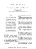
Figure 1: Bayesian sense induction model; shaded
nodes represent observed variables, unshaded
nodes indicate latent variables. Arrows indi-

cate conditional dependencies between variables,
whereas plates (the rectangles in the figure) refer
to repetitions of sampling steps. The variables in
the lower right corner refer to the number of sam-
ples.
consists of N
c
word tokens. We shall write φ
( j)
as a
shorthand for P(w
i
|s
i
= j), the multinomial distri-
bution over words for sense j, and θ
(c)
as a short-
hand for the distribution of senses in context c.
Following Blei et al. (2003) we will assume that
the mixing proportion over senses θ is drawn from
a Dirichlet prior with parameters α. The role of
the hyperparameter α is to create a smoothed sense
distribution. We also place a symmetric Dirichlet β
on φ (Griffiths and Steyvers, 2002). The hyper-
parmeter β can be interpreted as the prior observa-
tion count on the number of times context words
are sampled from a sense before any word from
the corpus is observed. Our model is represented
in graphical notation in Figure 1.

The model sketched above only takes word in-
formation into account. Methods developed for su-
pervised WSD often use a variety of information
sources based not only on words but also on lem-
mas, parts of speech, collocations and syntactic re-
lationships (Lee and Ng, 2002). The first idea that
comes to mind, is to use the same model while
treating various features as word-like elements. In
other words, we could simply assume that the con-
texts we wish to model are the union of all our
features. Although straightforward, this solution
is undesirable. It merges the distributions of dis-
tinct feature categories into a single one, and is
therefore conceptually incorrect, and can affect the
performance of the model. For instance, parts-of-
speech (which have few values, and therefore high
probability), would share a distribution with words
(which are much sparser). Layers containing more
elements (e.g. 10 word window) would overwhelm
105
α
θ
s
f
N
c
1
C
s
f

N
c
2
.
.
.
s
f
N
c
n
φ
1(β
1
)
φ
2(β
2
)
φ
n(β
n
)
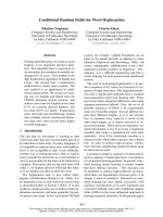
Figure 2: Extended sense induction model; inner
rectangles represent different sources (layers) of
information. All layers share the same, instance-
specific, sense distribution (θ), but each have their
own (multinomial) sense-feature distribution (φ).
Shaded nodes represent observed features f ; these
can be words, parts of speech, collocations or de-

pendencies.
smaller ones (e.g. 1 word window).
Our solution is to treat each information source
(or feature type) individually and then combine
all of them together in a unified model. Our un-
derlying assumption is that the context window
around the target word can have multiple represen-
tations, all of which share the same sense distribu-
tion. We illustrate this in Figure 2 where each inner
rectangle (layer) corresponds to a distinct feature
type. We will naively assume independence be-
tween multiple layers, even though this is clearly
not the case in our task. The idea here is to model
each layer as faithfully as possible to the empirical
data while at the same time combining information
from all layers in estimating the sense distribution
of each target instance.
4 Inference
Our inference procedure is based on Gibbs sam-
pling (Geman and Geman, 1984). The procedure
begins by randomly initializing all unobserved
random variables. At each iteration, each random
variable s
i
is sampled from the conditional distri-
bution P(s
i
|
s
−i

) where s
−i
refers to all variables
other than s
i
. Eventually, the distribution over sam-
ples drawn from this process will converge to the
unconditional joint distribution P(s) of the unob-
served variables (provided certain criteria are ful-
filled).
In our model, each element in each layer is a
variable, and is assigned a sense label (see Fig-
ure 2, where distinct layers correspond to differ-
ent representations of the context around the tar-
get word). From these assignments, we must de-
termine the sense distribution of the instance as a
whole. This is the purpose of the Gibbs sampling
procedure. Specifically, in order to derive the up-
date function used in the Gibbs sampler, we must
provide the conditional probability of the i-th vari-
able being assigned sense s
i
in layer l, given the
feature value f
i
of the context variable and the cur-
rent sense assignments of all the other variables in
the data (s
−i
):

p(s
i
|s
−i
, f ) ∝ p( f
i
|s, f
−i
, β) · p(s
i
|s
−i
, α) (2)
The probability of a single sense assignment, s
i
,
is proportional to the product of the likelihood (of
feature f
i
, given the rest of the data) and the prior
probability of the assignment.
(3)
p( f
i
|s, f
−i
, β) =
Z
p( f
i

|l, s, φ) · p(φ| f
−i
, β
l
)dφ =
#( f
i
, s
i
) +β
l
#(s
i
) +V
l
· β
l
For the likelihood term p( f
i
|s, f
−i
, β), integrating
over all possible values of the multinomial feature-
sense distribution φ gives us the rightmost term in
Equation 3, which has an intuitive interpretation.
The term #( f
i
, s
i
) indicates the number of times

the feature-value f
i
was assigned sense s
i
in the
rest of the data. Similarly, #(s
i
) indicates the num-
ber of times the sense assignment s
i
was observed
in the data. β
l
is the Dirichlet prior for the feature-
sense distribution φ in the current layer l, and V
l
is the size of the vocabulary of that layer, i.e., the
number of possible feature values in the layer. In-
tuitively, the probability of a feature-value given
a sense is directly proportional to the number of
times we have seen that value and that sense-
assignment together in the data, taking into ac-
count a pseudo-count prior, expressed through β.
This can also be viewed as a form of smoothing.
A similar approach is taken with regards to the
prior probability p(s
i
|s
−i
, α). In this case, how-

ever, all layers must be considered:
p(s
i
|s
−i
, α) =
∑
l
λ
l
· p(s
i
|l, s
−i
, α
l
) (4)
106
Here λ
l
is the weight for the contribution of layer l,
and α
l
is the portion of the Dirichlet prior for the
sense distribution θ in the current layer. Treating
each layer individually, we integrate over the pos-
sible values of θ, obtaining a similar count-based
term:
(5)
p(s

i
|l, s
−i
, α
l
) =
Z
p(s
i
|l, s
−i
, θ) · p(θ| f
−i
, α
l
)dθ =
#l(s
i
) +α
l
#l +S · α
l
where #l(s
i
) indicates the number of elements in
layer l assigned the sense s
i
, #l indicates the num-
ber of elements in layer l, i.e., the size of the layer
and S the number of senses.

To distribute the pseudo counts represented by
α in a reasonable fashion among the layers, we
define α
l
=
#l
#m
· α where #m =
∑
l
#l, i.e., the total
size of the instance. This distributes α according
to the relative size of each layer in the instance.
p(s
i
|l,
s
−i
, α
l
)=
#l(s
i
) +
#l
#m
· α
#l +S ·
#l
#m

· α
=
#m ·
#l(s
i
)
#l
+ α
#m +S · α
(6)
Placing these values in Equation 4 we obtain the
following:
p(s
i
|s
−i
, α) =
#m ·
∑
l
λ
l
·
#l(s
i
)
#l
+ α
#m +S · α
(7)

Putting it all together, we arrive at the final update
equation for the Gibbs sampling:
p(s
i
|s
−i
, f )∝
#( f
i
, s
i
) +β
l
#(s
i
) +V
l
· β
l
·
#m ·
∑
l
λ
l
·
#l(s
i
)
#l

+ α
#m +S · α
(8)
Note that when dealing with a single layer, Equa-
tion 8 collapses to:
p(s
i
|s
−i
, f ) ∝
#( f
i
, s
i
) +β
#(s
i
) +V · β
·
#m(s
i
) +α
#m +S · α
(9)
where #m(s
i
) indicates the number of elements
(e.g., words) in the context window assigned to
sense s
i

. This is identical to the update equation
in the original, word-based LDA model.
The sampling algorithm gives direct estimates
of s for every context element. However, in view
of our task, we are more interested in estimating θ,
the sense-context distribution which can be ob-
tained as in Equation 7, but taking into account
all sense assignments, without removing assign-
ment i. Our system labels each instance with the
single, most probable sense.
5 Evaluation Setup
In this section we discuss our experimental set-up
for assessing the performance of the model pre-
sented above. We give details on our training pro-
cedure, describe our features, and explain how our
system output was evaluated.
Data In this work, we focus solely on inducing
senses for nouns, since they constitute the largest
portion of content words. For example, nouns rep-
resent 45% of the content words in the British Na-
tional Corpus. Moreover, for many tasks and ap-
plications (e.g., web queries, Jansen et al. 2000)
nouns are the most frequent and most important
part-of-speech.
For evaluation, we used the Semeval-2007
benchmark dataset released as part of the sense
induction and discrimination task (Agirre and
Soroa, 2007). The dataset contains texts from the
Penn Treebank II corpus, a collection of articles
from the first half of the 1989 Wall Street Jour-

nal (WSJ). It is hand-annotated with OntoNotes
senses (Hovy et al., 2006) and has 35 nouns. The
average noun ambiguity is 3.9, with a high (almost
80%) skew towards the predominant sense. This is
not entirely surprising since OntoNotes senses are
less fine-grained than WordNet senses.
We used two corpora for training as we wanted
to evaluate our model’s performance across differ-
ent domains. The British National Corpus (BNC)
is a 100 million word collection of samples of
written and spoken language from a wide range of
sources including newspapers, magazines, books
(both academic and fiction), letters, and school es-
says as well as spontaneous conversations. This
served as our out-of-domain corpus, and con-
tained approximately 730 thousand instances of
the 35 target nouns in the Semeval lexical sample.
The second, in-domain, corpus was built from se-
lected portions of the Wall Street Journal. We used
all articles (excluding the Penn Treebank II por-
tion used in the Semeval dataset) from the years
1987-89 and 1994 to create a corpus of similar size
to the BNC, containing approximately 740 thou-
sand instances of the target words.
Additionally, we used the Senseval 2 and 3 lex-
ical sample data (Preiss and Yarowsky, 2001; Mi-
halcea and Edmonds, 2004) as development sets,
for experimenting with the hyper-parameters of
our model (see Section 6).
Evaluation Methodology Agirre and Soroa

(2007) present two evaluation schemes for as-
sessing sense induction methods. Under the first
107
scheme, the system output is compared to the
gold standard using standard clustering evalua-
tion metrics (e.g., purity, entropy). Here, no at-
tempt is made to match the induced senses against
the labels of the gold standard. Under the second
scheme, the gold standard is partitioned into a test
and training corpus. The latter is used to derive a
mapping of the induced senses to the gold stan-
dard labels. The mapping is then used to calculate
the system’s F-Score on the test corpus.
Unfortunately, the first scheme failed to dis-
criminate among participating systems. The one-
cluster-per-word baseline outperformed all sys-
tems, except one, which was only marginally bet-
ter. The scheme ignores the actual labeling and
due to the dominance of the first sense in the data,
encourages a single-sense approach which is fur-
ther amplified by the use of a coarse-grained sense
inventory. For the purposes of this work, there-
fore, we focused on the second evaluation scheme.
Here, most of the participating systems outper-
formed the most-frequent-sense baseline, and the
rest obtained only slightly lower scores.
Feature Space Our experiments used a feature
set designed to capture both immediate local con-
text, wider context and syntactic context. Specifi-
cally, we experimented with six feature categories:

±10-word window (10w), ±5-word window (5w),
collocations (1w), word n-grams (ng), part-of-
speech n-grams (pg) and dependency relations
(dp). These features have been widely adopted in
various WSD algorithms (see Lee and Ng 2002 for
a detailed evaluation). In all cases, we use the lem-
matized version of the word(s).
The Semeval workshop organizers provided a
small amount of context for each instance (usu-
ally a sentence or two surrounding the sentence
containing the target word). This context, as well
as the text in the training corpora, was parsed us-
ing RASP (Briscoe and Carroll, 2002), to extract
part-of-speech tags, lemmas, and dependency in-
formation. For instances containing more than one
occurrence of the target word, we disambiguate
the first occurrence. Instances which were not cor-
rectly recognized by the parser (e.g., a target word
labeled with the wrong lemma or part-of-speech),
were automatically assigned to the largest sense-
cluster.
3
3
This was the case for less than 1% of the instances.
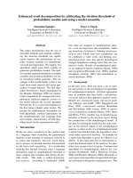
3 4
5 6
7
8 9
Number of Senses
83

84
85
86
87
88
F-Score (%)
In-Domain (WSJ)
Out-of-Domain (BNC)
Figure 3: Model performance with varying num-
ber of senses on the WSJ and BNC corpora.
6 Experiments
Model Selection The framework presented in
Section 3 affords great flexibility in modeling the
empirical data. This however entails that several
parameters must be instantiated. More precisely,
our model is conditioned on the Dirichlet hyper-
parameters α and β and the number of senses S.
Additional parameters include the number of iter-
ations for the Gibbs sampler and whether or not
the layers are assigned different weights.
Our strategy in this paper is to fix α and β
and explore the consequences of varying S. The
value for the α hyperparameter was set to 0.02.
This was optimized in an independent tuning ex-
periment which used the Senseval 2 (Preiss and
Yarowsky, 2001) and Senseval 3 (Mihalcea and
Edmonds, 2004) datasets. We experimented with
α values ranging from 0.005 to 1. The β parame-
ter was set to 0.1 (in all layers). This value is often
considered optimal in LDA-related models (Grif-

fiths and Steyvers, 2002). For simplicity, we used
uniform weights for the layers. The Gibbs sampler
was run for 2,000 iterations. Due to the random-
ized nature of the inference procedure, all reported
results are average scores over ten runs.
Our experiments used the same number of
senses for all the words, since tuning this number
individually for each word would be prohibitive.
We experimented with values ranging from three
to nine senses. Figure 3 shows the results obtained
for different numbers of senses when the model is
trained on the WSJ (in-domain) and BNC (out-of-
domain) corpora, respectively. Here, we are using
the optimal combination of layers for each system
(which we discuss in the following section in de-
108
Senses of drug (WSJ)
1. U.S., administration, federal, against, war, dealer
2. patient, people, problem, doctor, company, abuse
3. company, million, sale, maker, stock, inc.
4. administration, food, company, approval, FDA
Senses of drug (BNC)
1. patient, treatment, effect, anti-inflammatory
2. alcohol, treatment, patient, therapy, addiction
3. patient, new, find, effect, choice, study
4. test, alcohol, patient, abuse, people, crime
5. trafficking, trafficker, charge, use, problem
6. abuse, against, problem, treatment, alcohol
7. people, wonder, find, prescription, drink, addict
8. company, dealer, police, enforcement, patient

Table 1: Senses inferred for the word drug from
the WSJ and BNC corpora.
tail). For the model trained on WSJ, performance
peaks at four senses, which is similar to the av-
erage ambiguity in the test data. For the model
trained on the BNC, however, the best results are
obtained using twice as many senses. Using fewer
senses with the BNC-trained system can result in
a drop in accuracy of almost 2%. This is due to
the shift in domain. As the sense-divisions of the
learning domain do not match those of the target
domain, finer granularity is required in order to en-
compass all the relevant distinctions.
Table 1 illustrates the senses inferred for the
word drug when using the in-domain and out-of-
domain corpora, respectively. The most probable
words for each sense are also shown. Firstly, note
that the model infers some plausible senses for
drug on the WSJ corpus (top half of Table 1).
Sense 1 corresponds to the “enforcement” sense
of drug, Sense 2 refers to “medication”, Sense 3
to the “drug industry” and Sense 4 to “drugs re-
search”. The inferred senses for drug on the BNC
(bottom half of Table 1) are more fine grained. For
example, the model finds distinct senses for “med-
ication” (Sense 1 and 7) and “illegal substance”
(Senses 2, 4, 6, 7). It also finds a separate sense
for “drug dealing” (Sense 5) and “enforcement”
(Sense 8). Because the BNC has a broader fo-
cus, finer distinctions are needed to cover as many

senses as possible that are relevant to the target do-
main (WSJ).
Layer Analysis We next examine which indi-
vidual feature categories are most informative
in our sense induction task. We also investigate
whether their combination, through our layered
1-Layer
10w 86.9
5w 86.8
1w 84.6
ng 83.6
pg 82.5
dp 82.2
MFS 80.9
5-Layers
-10w 83.1
-5w 83.0
-1w 83.0
-ng 83.0
-pg 82.7
-dp 84.7
all 83.3
Combination
10w+5w 87.3%
5w+pg 83.9%
1w+ng 83.2%
10w+pg 83.3%
1w+pg 84.5%
10w+pg+dep 82.2%
MFS 80.9%

Table 2: Model performance (F-score) on the WSJ
with one layer (left), five layers (middle), and se-
lected combinations of layers (right).
model (see Figure 2), yields performance im-
provements. We used 4 senses for the system
trained on WSJ and 8 for the system trained on
the BNC (α was set to 0.02 and β to 0.1)
Table 2 (left side) shows the performance of our
model when using only one layer. The layer com-
posed of words co-occurring within a ±10-word
window (10w), and representing wider, topical, in-
formation gives the highest scores on its own. It
is followed by the ±5 (5w) and ±1 (1w) word
windows, which represent more immediate, local
context. Part-of-speech n-grams (pg) and word n-
grams (ng), on their own, achieve lower scores,
largely due to over-generalization and data sparse-
ness, respectively. The lowest-scoring single layer
is the dependency layer (dp), with performance
only slightly above the most-frequent-sense base-
line (MFS). Dependency information is very infor-
mative when present, but extremely sparse.
Table 2 (middle) also shows the results obtained
when running the layered model with all but one
of the layers as input. We can use this informa-
tion to determine the contribution of each layer by
comparing to the combined model with all layers
(all). Because we are dealing with multiple lay-
ers, there is an element of overlap involved. There-
fore, each of the word-window layers, despite rel-

atively high informativeness on its own, does not
cause as much damage when it is absent, since
the other layers compensate for the topical and lo-
cal information. The absence of the word n-gram
layer, which provides specific local information,
does not make a great impact when the 1w and pg
layers are present. Finally, we can see that the ex-
tremely sparse dependency layer is detrimental to
the multi-layer model as a whole, and its removal
increases performance. The sparsity of the data in
this layer means that there is often little informa-
tion on which to base a decision. In these cases,
the layer contributes a close-to-uniform estimation
109
1-Layer
10w 84.6
5w 84.6
1w 83.6
pg 83.1
ng 82.8
dp 81.1
MFS 80.9
5-Layers
-10w 83.3
-5w 82.8
-1w 83.5
-pg 83.2
-ng 82.9
-dp 84.7
all 84.1

Combination
10w+5w 85.5%
5w+pg 83.5%
1w+ng 83.5%
10w+pg 83.4%
1w+pg 84.1%
10w+pg+dep 81.7%
MFS 80.9%
Table 3: Model performance (F-score) on the BNC
with one layer (left), five layers (middle), and se-
lected combinations of layers (right).
of the sense distribution, which confuses the com-
bined model.
Other layer combinations obtained similar re-
sults. Table 2 (right side) shows the most informa-
tive two and three layer combinations. Again, de-
pendencies tend to decrease performance. On the
other hand, combining features that have similar
performance on their own is beneficial. We obtain
the best performance overall with a two layered
model combining topical (+10w) and local (+5w)
contexts.
Table 3 replicates the same suite of experiments
on the BNC corpus. The general trends are similar.
Some interesting differences are apparent, how-
ever. The sparser layers, notably word n-grams
and dependencies, fare comparatively worse. This
is expected, since the more precise, local, infor-
mation is likely to vary strongly across domains.
Even when both domains refer to the same sense

of a word, it is likely to be used in a different
immediate context, and local contextual informa-
tion learned in one domain will be less effective
in the other. Another observable difference is that
the combined model without the dependency layer
does slightly better than each of the single layers.
The 1w+pg combination improves over its compo-
nents, which have similar individual performance.
Finally, the best performing model on the BNC
also combines two layers capturing wider (10w)
and more local (5w) contextual information (see
Table 3, right side).
Comparison to State-of-the-Art Table 4 com-
pares our model against the two best performing
sense induction systems that participated in the
Semeval-2007 competition. IR2 (Niu et al., 2007)
performed sense induction using the Information
Bottleneck algorithm, whereas UMND2 (Peder-
sen, 2007) used k-means to cluster second order
co-occurrence vectors associated with the target
System F-Score
10w, 5w (WSJ) 87.3
I2R 86.8
UMND2 84.5
MFS 80.9
Table 4: Comparison of the best-performing
Semeval-07 systems against our model.
word. These models and our own model signif-
icantly outperform the most-frequent-sense base-
line (p < 0.01 using a χ

2
test). Our best sys-
tem (10w+5w on WSJ) is significantly better than
UMND2 (p < 0.01) and quantitatively better than
IR2, although the difference is not statistically sig-
nificant.
7 Discussion
This paper presents a novel Bayesian approach to
sense induction. We formulated sense induction
in a generative framework that describes how the
contexts surrounding an ambiguous word might
be generated on the basis of latent variables. Our
model incorporates features based on lexical in-
formation, parts of speech, and dependencies in a
principled manner, and outperforms state-of-the-
art systems. Crucially, the approach is not specific
to the sense induction task and can be adapted for
other applications where it is desirable to take mul-
tiple levels of information into account. For exam-
ple, in document classification, one could consider
an accompanying image and its caption as possi-
ble additional layers to the main text.
In the future, we hope to explore more rigor-
ous parameter estimation techniques. Goldwater
and Griffiths (2007) describe a method for inte-
grating hyperparameter estimation into the Gibbs
sampling procedure using a prior over possible
values. Such an approach could be adopted in our
framework, as well, and extended to include the
layer weighting parameters, which have strong po-

tential for improving the model’s performance. In
addition, we could allow an infinite number of
senses and use an infinite Dirichlet model (Teh
et al., 2006) to automatically determine how many
senses are optimal. This provides an elegant so-
lution to the model-order problem, and eliminates
the need for external cluster-validation methods.
Acknowledgments The authors acknowledge
the support of EPSRC (grant EP/C538447/1).
We are grateful to Sharon Goldwater for her feed-
back on earlier versions of this work.
110
References
Agirre, Eneko, Llu
´
ıs M
`
arquez, and Richard Wicentowski, ed-
itors. 2007. Proceedings of the SemEval-2007. Prague,
Czech Republic.
Agirre, Eneko and Aitor Soroa. 2007. Semeval-2007 task
02: Evaluating word sense induction and discrimination
systems. In Proceedings of SemEval-2007. Prague, Czech
Republic, pages 7–12.
Barnard, K., P. Duygulu, D. Forsyth, N. De Freitas, D. M.
Blei, and M. I. Jordan. 2003. Matching words and pictures.
J. of Machine Learning Research 3(6):1107–1135.
Blei, David M., Andrew Y. Ng, and Michael I. Jordan. 2003.
Latent dirichlet allocation. Journal of Machine Learning
Research 3:993–1022.

Bordag, Stefan. 2006. Word sense induction: Triplet-based
clustering and automatic evaluation. In Proceedings of the
11th EACL. Trento, Italy, pages 137–144.
Boyd-Graber, Jordan and David Blei. 2007. Putop: Turning
predominant senses into a topic model for word sense dis-
ambiguation. In Proceedings of SemEval-2007. Prague,
Czech Republic, pages 277–281.
Boyd-Graber, Jordan, David Blei, and Xiaojin Zhu. 2007.
A topic model for word sense disambiguation. In Pro-
ceedings of the EMNLP-CoNLL. Prague, Czech Republic,
pages 1024–1033.
Briscoe, Ted and John Carroll. 2002. Robust accurate statis-
tical annotation of general text. In Proceedings of the 3rd
LREC. Las Palmas, Gran Canaria, pages 1499–1504.
Cai, J. F., W. S. Lee, and Y. W. Teh. 2007. Improving word
sense disambiguation using topic features. In Proceedings
of the EMNLP-CoNLL. Prague, Czech Republic, pages
1015–1023.
Carpuat, Marine and Dekai Wu. 2005. Word sense disam-
biguation vs. statistical machine translation. In Proceed-
ings of the 43rd ACL. Ann Arbor, MI, pages 387–394.
Dorow, Beate and Dominic Widdows. 2003. Discovering
corpus-specific word senses. In Proceedings of the 10th
EACL. Budapest, Hungary, pages 79–82.
Firth, J. R. 1957. A Synopsis of Linguistic Theory 1930-1955.
Oxford: Philological Society.
Gauch, Susan and Robert P. Futrelle. 1993. Experiments in
automatic word class and word sense identification for in-
formation retrieval. In Proceedings of the 3rd Annual Sym-
posium on Document Analysis and Information Retrieval.

Las Vegas, NV, pages 425–434.
Geman, S. and D. Geman. 1984. Stochastic relaxation, Gibbs
distribution, and Bayesian restoration of images. IEEE
Transactions on Pattern Analysis and Machine Intelli-
gence 6(6):721–741.
Goldwater, Sharon and Tom Griffiths. 2007. A fully Bayesian
approach to unsupervised part-of-speech tagging. In Pro-
ceedings of the 45th ACL. Prague, Czech Republic, pages
744–751.
Griffiths, Thomas L., Mark Steyvers, David M. Blei, and
Joshua B. Tenenbaum. 2005. Integrating topics and syn-
tax. In Lawrence K. Saul, Yair Weiss, and L
´
eon Bottou,
editors, Advances in Neural Information Processing Sys-
tems 17, MIT Press, Cambridge, MA, pages 537–544.
Griffiths, Tom L. and Mark Steyvers. 2002. A probabilistic
approach to semantic representation. In Proeedings of the
24th Annual Conference of the Cognitive Science Society.
Fairfax, VA, pages 381–386.
Hovy, Eduard, Mitchell Marcus, Martha Palmer, Lance
Ramshaw, and Ralph Weischedel. 2006. Ontonotes: The
90% solution. In Proceedings of the HLT, Companion Vol-
ume: Short Papers. Association for Computational Lin-
guistics, New York City, USA, pages 57–60.
Jansen, B. J., A. Spink, and A. Pfaff. 2000. Linguistic aspects
of web queries.
Lee, Yoong Keok and Hwee Tou Ng. 2002. An empirical
evaluation of knowledge sources and learning algorithms
for word sense disambiguation. In Proceedings of the

EMNLP. Morristown, NJ, USA, pages 41–48.
McCarthy, Diana, Rob Koeling, Julie Weeds, and John Car-
roll. 2004. Finding predominant senses in untagged text.
In Proceedings of the 42nd ACL. Barcelona, Spain, pages
280–287.
Mihalcea, Rada and Phil Edmonds, editors. 2004. Proceed-
ings of the SENSEVAL-3. Barcelona.
Niu, Zheng-Yu, Dong-Hong Ji, and Chew-Lim Tan. 2007.
I2r: Three systems for word sense discrimination, chinese
word sense disambiguation, and english word sense dis-
ambiguation. In Proceedings of the Fourth International
Workshop on Semantic Evaluations (SemEval-2007). As-
sociation for Computational Linguistics, Prague, Czech
Republic, pages 177–182.
Pantel, Patrick and Dekang Lin. 2002. Discovering word
senses from text. In Proceedings of the 8th KDD. New
York, NY, pages 613–619.
Pedersen, Ted. 2007. Umnd2 : Senseclusters applied to the
sense induction task of senseval-4. In Proceedings of
SemEval-2007. Prague, Czech Republic, pages 394–397.
Preiss, Judita and David Yarowsky, editors. 2001. Proceed-
ings of the 2nd International Workshop on Evaluating
Word Sense Disambiguation Systems. Toulouse, France.
Purandare, Amruta and Ted Pedersen. 2004. Word sense dis-
crimination by clustering contexts in vector and similarity
spaces. In Proceedings of the CoNLL. Boston, MA, pages
41–48.
Sch
¨
utze, Hinrich. 1998. Automatic word sense discrimina-

tion. Computational Linguistics 24(1):97–123.
Teh, Y. W., M. I. Jordan, M. J. Beal, and D. M. Blei. 2006.
Hierarchical Dirichlet processes. Journal of the American
Statistical Association 101(476):1566–1581.
V
´
eronis, Jean. 2004. Hyperlex: lexical cartography for
information retrieval. Computer Speech & Language
18(3):223–252.
Vickrey, David, Luke Biewald, Marc Teyssier, and Daphne
Koller. 2005. Word-sense disambiguation for machine
translation. In Proceedings of the HLT/EMNLP. Vancou-
ver, pages 771–778.
Voorhees, Ellen M. 1993. Using wordnet to disambiguate
word senses for text retrieval. In Proceedings of the 16th
SIGIR. New York, NY, pages 171–180.
111