Tài liệu Báo cáo khoa học: "The Problem with Kappa" pdf

Proceedings of the 13th Conference of the European Chapter of the Association for Computational Linguistics, pages 345–355,
Avignon, France, April 23 - 27 2012.
c
2012 Association for Computational Linguistics


The Problem with Kappa


David M W Powers
Centre for Knowledge & Interaction Technology, CSEM
Flinders University







Abstract
It is becoming clear that traditional
evaluation measures used in
Computational Linguistics (including
Error Rates, Accuracy, Recall, Precision
and F-measure) are of limited value for
unbiased evaluation of systems, and are
not meaningful for comparison of
algorithms unless both the dataset and
algorithm parameters are strictly
controlled for skew (Prevalence and
Bias). The use of techniques originally

designed for other purposes, in particular
Receiver Operating Characteristics Area
Under Curve, plus variants of Kappa,
have been proposed to fill the void.
This paper aims to clear up some of the
confusion relating to evaluation, by
demonstrating that the usefulness of each
evaluation method is highly dependent on
the assumptions made about the
distributions of the dataset and the
underlying populations. The behaviour of
a number of evaluation measures is
compared under common assumptions.
Deploying a system in a context which
has the opposite skew from its validation
set can be expected to approximately
negate Fleiss Kappa and halve Cohen
Kappa but leave Powers Kappa
unchanged. For most performance
evaluation purposes, the latter is thus
most appropriate, whilst for comparison
of behaviour, Matthews Correlation is
recommended.
Introduction
Research in Computational Linguistics usually
requires some form of quantitative evaluation. A
number of traditional measures borrowed from
Information Retrieval (Manning & Schütze,
1999) are in common use but there has been
considerable critical evaluation of these measures

themselves over the last decade or so (Entwisle
& Powers, 1998, Flach, 2003, Ben-David. 2008).
Receiver Operating Analysis (ROC) has been
advocated as an alternative by many, and in
particular has been used by Fürnkranz and Flach
(2005), Ben-David (2008) and Powers (2008) to
better understand both learning algorithms
relationship and the between the various
measures, and the inherent biases that make
many of them suspect. One of the key advantages
of ROC is that it provides a clear indication of
chance level performance as well as a less well
known indication of the relative cost weighting
of positive and negative cases for each possible
system or parameterization represented.
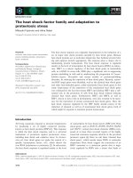
ROC Area Under the Curve (Fig. 1) has been
also used as a performance measure but averages
over the false positive rate (Fallout) and is thus a
function of cost that is dependent on the
classifier rather than the application. For this
reason it has come into considerable criticism
and a number of variants and alternatives have
been proposed (e.g. AUK, Kaymak et. Al, 2010
and H-measure, Hand, 2009). An AUC curve
that is at least as good as a second curve at all
points, is said to dominate it and indicates that
the first classifier is equal or better than the
second for all plotted values of the parameters,
and all cost ratios. However AUC being greater
for one classifier than another does not have such

a property – indeed deconvexities within or
345


intersections of ROC curves are both prima facie
evidence that fusion of the parameterized
classifiers will be useful (cf. Provost and Facett,
2001; Flach and Wu, 2005).
AUK stands for Area under Kappa, and
represents a step in the advocacy of Kappa (Ben-
David, 2008ab) as an alternative to the traditional
measures and ROC AUC. Powers (2003,2007)
has also proposed a Kappa-like measure
(Informedness) and analysed it in terms of ROC,
and there are many more, Warrens (2010) analyzing
the relationships between some of the others.
Systems like RapidMiner (2011) and Weka
(Witten and Frank, 2005) provide almost all of
the measures we have considered, and many
more besides. This encourages the use of
multiple measures, and indeed it is now
becoming routine to display tables of multiple
results for each system, and this is in particular
true for the frameworks of some of the
challenges and competitions brought to the
communities (e.g. 2
nd
i2b2 Challenge in NLP for
Clinical Data, 2011; 2
nd

Pascal Challenge on
HTC, 2011)).
This use of multiple statistics is no doubt in
response to the criticism levelled at the
evaluation mechanisms used in earlier
generations of competitions and the above
mentioned critiques, but the proliferation of
alternate measures in some ways merely
compounds the problem. Researchers have the
temptation of choosing those that favour their
system as they face the dilemma of what to do
about competing (and often disagreeing)
evaluation measures that they do not completely
understand. These systems and competitions also
exhibit another issue, the tendency to macro-
averages over multiple classes, even of measures
that are not denominated in class (e.g. that are
proportions of predicted labels rather than real
classes, as with Precision).
This paper is directed at better understanding
some of these new and old measures as well as
providing recommendations as to which measures
are appropriate in which circumstances.
What’s in a Kappa?
In this paper we focus on the Kappa family of
measures, as well as some closely related
statistics named for other letters of the Greek
alphabet, and some measures that we will show
behave as Kappa measures although they were
not originally defined as such. These include

Informedness, Gini Coefficient and single point
ROC AUC, which are in fact all equivalent to
DeltaP’ in the dichotomous case, which we deal
with first, and to the other Kappas when the
marginal prevalences (or biases) match.
1.1 Two classes and non-negative Kappa.
Kappa was originally proposed (Cohen, 1960) to
compare human ratings in a binary, or
dichotomous, classification task. Cohen (1960)
recognized that Rand Accuracy did not take
chance into account and therefore proposed to
subtract off the chance level of Accuracy and
then renormalize to the form of a probability:
K(Acc) = [Acc – E(Acc)] / [1 – E(Acc)] (1)
This leaves the question of how to estimate the
expected Accuracy, E(Acc). Cohen (1960) made
the assumption that raters would have different
distributions that could be estimated as
the products of the corresponding marginal
coefficients of the contingency table:


+ve Class
−ve Class

+ve Prediction
A=TP
B=FP
PP
−ve Prediction

C=FN
D=TN
PN
Notation
RP
RN
N
Table 1. Statistical and IR Contingency Notation
In order to discuss this further it is important
to discuss our notational conventions, and it is
noted that in statistics, the letters A-D (upper
case or lower case) are conventionally used to
label the cells, and their sums may be used to
label the marginal cells. However in the
literature on ROC analysis, which we follow
here, it is usual to talk about true and false
positives (that is positive predictions that are
correct or incorrect), and conversely true and
false negatives. Often upper case is used to
indicate counts in the contingency table, which
sum to the number of instances, N. In this case
lower case letters are used to indicate
probabilities, which means that the
corresponding upper case values in the
contingency table are all divided by N, and n=1.
Statistics relative to (the total numbers of
items in) the real classes are called Rates and
have the number (or proportion) of Real
Positives (RP) or Real Negatives (RN) in the
denominator. In this notation, we have Recall =

TPR = TP/RP.
Conversely statistics relative to the (number
of) predictions are called Accuracies, so relative
to the predictions that label instances positively,
Predicted Positives (PP), we have Precision =
TPA = TP/PP.
346


The accuracy of all our predictions, positive or
negative, is given by Rand Accuracy =
(TF+TN)/N = tf+tn, and this is what is meant in
general by the unadorned term Accuracy, or the
abbreviation Acc.
Rand Accuracy is the weighted average of
Precision and Inverse Precision (probability that
negative predictions are correctly labeled), where
the weighting is made according to the number
of predictions made for the corresponding labels.
Rand Accuracy is also the weighted average of
Recall and Inverse Recall (probability that
negative instances are correctly predicted),
where the weighting is made according to the
number of instances in the corresponding
classes.
The marginal probabilities rp and pp are also
known as Prevalence (the class prevalence of
positive instances) and Bias (the label bias to
positive predictions), and the corresponding
probabilities of negative classes and labels are

the Inverse Prevalence and Inverse Bias
respectively. In the ROC literature, the ratios of
negative to positive classes is often referred to as
the class ratio or skew. We can similarly also
refer to a label ratio, prediction ratio or
prediction skew. Note that optimal performance
can only be achieved if class skew = label skew.
The Expected True Positives and Expected
True Negatives for Cohen Kappa, as well as Chi-
squared significance, are estimated as the
product of Bias and Prevalence, and the product
of Inverse Bias and Inverse Prevalence, resp.,
where traditional uses of Kappa for agreement of
human raters, the contingency table represents
one rater as providing the classification to be
predicted by the other rater. Cohen assumes that
their distribution of ratings are independent, as
reflected both by the margins and the
contingencies: ETP = RP*PP; ETN = RN*NN.
This gives us E(Acc) = (ETP+ETN)/N=etp+etn.
By contrast the two rater two class form of
Fleiss (1981) Kappa, also known as Scott Pi,
assumes that both raters are labeling
independently using the same distribution, and
that the margins reflect this potential variation.
The expected number of positives is thus
effectively estimated as the average of the two
raters’ counts, so that EP = (RP+PP)/2, and EN =
(RN+PN)/2, ETP = EP
2

and ETN = EN
2
.
1.2 Inverting Kappa
The definition of Kappa in Eqn (1) can be seen
to be applicable to arbitrary definitions of
Expected Accuracy, and in order to discover how
other measures relate to the family of Kappa
measures it is useful to invert Kappa to discover
the implicit definition of Expected Accuracy that
allows a measure to be interpreted as a form of
Kappa. We simply make E(Acc) the subject by
multiplying out Eqn (1) to a common
denominator and associating factors of E(Acc):


Figure 1. Illustration of ROC Analysis. The
solid diagonal represents chance performance
for different rates of guessing positive or
negative labels. The dotted line represent the
convex hull enclosing the results of different
systems, thresholds or parameters tested. The
(0,0) and (1,1) points represent guessing always
negative and always positive and are always
nominal systems in a ROC curve. The points
along any straight line segment of a convex hull
are achievable by probabilistic interpolation of
the systems at each end, the gradient represents
the cost ratio and all points along the segment,
including the endpoints have the same effective

cost benefit. AUC is the area under the curve
joining the systems with straight edges and
AUCH is the area under the convex hull where
points within it are ignored. The height above
the chance line of any point represents DeltaP’,
the Gini Coefficient and also the Dichotomous
Informedness of the corresponding system, and
also corresponds to twice the area of the triangle
between it and the chance line, and thus 2AUC-1
where AUC is calculated on this single point
curve (not shown) joining it to (0,0) and (1,1).
The (1,0) point represents perfect performance
with 100% True Positive Rate and 0% False
Negative Rate.
!
347


K(Acc) = [Acc – E(Acc)] / [1 – E(Acc)] (1)
E(Acc) = [Acc – K(Acc)] / [1 – K(Acc)] (2)
Note that for a given value of Acc the function
connecting E(Acc) and K(Acc) is its own
inverse:
E(Acc) = f
Acc
(K(Acc)) (3)
K(Acc) = f
Acc
(E(Acc)) (4)
For the future we will tend to drop the Acc

argument or subscript when it is clear, and we
will also subscript E and K with the name or
initial of the corresponding definition of
Expectation and thus Kappa (viz. Fleiss and
Cohen so far).
Note that given Acc and E(Acc) are in the
range of 0 1 as probabilities, Kappa is also
restricted to this range, and takes the form of a
probability.
1.3 Multiclass multirater Kappa
Fleiss (1981) and others sought to generalize the
Cohen (1960) definition of Kappa to handle both
multiple class (not just positive/negative) and
multiple raters (not just two – one of which we
have called real and the other prediction). Fleiss
in fact generalized Scott’s (1955) Pi in both
senses, not Cohen Kappa. The Fleiss Kappa is
not formulated as we have done here for
exposition, but in terms of pairings (agreements)
amongst the raters, who are each assumed to
have rated the same number of items, N, but not
necessarily all. Krippendorf’s (1970, 1978)
effectively generalizes further by dealing with
arbitrary numbers of raters assessing different
numbers of items.
Light (1971) and Hubert (1977) successfully
generalized Cohen Kappa. Another approach to
estimating E(Acc) was taken by Bennett et al
(1955) which basically assumed all classes were
equilikely (effectively what use of Accuracy, F-

Measure etc. do, although they don’t subtract off
the chance component).
The Bennett Kappa was generalized by
Randolph (2005), but as our starting point is that
we need to take the actual margins into account,
we do not pursue these further. However,
Warrens (2010a) shows that, under certain
conditions, Fleiss Kappa is a lower bound of
both the Hubert generalization of Cohen Kappa
and the Randolph generalization of Bennet
Kappa, which is itself correspondingly an upper
bound of both the Hubert and the Light
generalizations of Cohen Kappa. Unfortunately
the conditions are that there is some agreement
between the class and label skews (viz. the
prevalence and bias of each class/label). Our
focus in this paper is the behaviour of the various
Kappa measures as we move from strongly
matched to strongly mismatched biases.
Cohen (1968) also introduced a weighted
variant of Kappa. We have also discussed cost
weighting in the context of ROC, and Hand
(2009) seeks to improve on ROC AUC by
introducing a beta distribution as an estimated
cost profile, but we will not discuss them further
here as we are more interested in the
effectiveness of the classifer overall rather than
matching a particular cost profile, and are
skeptical about any generic cost distribution. In
particular the beta distribution gives priority to

central tendency rather than boundary conditions,
but boundary conditions are frequently
encountered in optimization. Similarly Kaymak
et al.’s (2010) proposal to replace AUC by AUK
corresponds to a Cohen Kappa reweighting of
ROC that eliminates many of its useful
properties, without any expectation that the
measure, as an integration across a surrogate cost
distribution, has any validity for system
selection. Introducing alternative weights is also
allowed in the definition of F-Measure, although
in practice this is almost invariably employed as
the equally weighted harmonic mean of Recall
and Precision. Introducing additional weight or
distribution parameters, just multiplies the
confusion as to which measure to believe.
Powers (2003) derived a further multiclass
Kappa-like measure from first principles,
dubbing it Informedness, based on an analogy of
Bookmaker associating costs/payoffs based on
the odds. This is then proven to measure the
proportion of time (or probability) a decision is
informed versus random, based on the same
assumptions re expectation as Cohen Kappa, and
we will thus call it Powers Kappa, and derive an
formulation of the corresponding expectation.
Powers (2007) further identifies that the
dichotomous form of Powers Kappa is equivalent
to the Gini cooefficient as a deskewed version of
the weighted Relative Accuracy proposed by

Flach (2003) based on his analysis and
deskewing of common evaluation measures in
the ROC paradigm. Powers (2007) also identifies
that Dichotomous Informedness is equivalent to
an empirically derived psychological measure
called DeltaP’ (Perruchet et al. 2004). DeltaP’
(and its dual DeltaP) were derived based on
analysis of human word association data – the
combination of this empirical observation with
the place of DeltaP’ as the dichotomous case of
348


Powers’ ‘Informedness’ suggests that human
association is in some sense optimal. Powers
(2007) also introduces a dual of Informedness
that he names Markedness, and shows that the
geometric mean of Informedness and
Markedness is Matthews Correlation, the
nominal analog of Pearson Correlation.
Powers’ Informedness is in fact a variant of
Kappa with some similarities to Cohen Kappa,
but also some advantages over both Cohen and
Fleiss Kappa due to its asymmetric relation with
Recall, in the dichotomous form of Powers (2007),
Informedness = Recall + InverseRecall – 1
= (Recall – Bias) / (1 – Prevalence).
If we think of Kappa as assessing the
relationship between two raters, Powers’ statistic
is not evenhanded and the Informedness and

Markedness duals measure the two directions of
prediction, normalizing Recall and Precision. In
fact, the relationship with Correlation allows
these to be interpreted as regression coefficients
for the prediction function and its inverse.
1.4 Kappa vs Correlation
It is often asked why we don’t just use
Correlation to measure. In fact, Castellan (1996)
uses Tetrachoric Correlation, another
generalization of Pearson Correlation that
assumes that the two class variables are given by
underlying normal distributions. Uebersax
(1987), Hutchison (1993) and Bonnet and Price
(2005) each compare Kappa and Correlation and
conclude that there does not seem to be any
situation where Kappa would be preferable to
Correlation. However all the Kappa and
Correlation variants considered were symmetric,
and it is thus interesting to consider the separate
regression coefficients underlying it that
represent the Powers Kappa duals of
Informedness and Markedness, which have the
advantage of separating out the influences of
Prevalence and Bias (which then allows macro-
averaging, which is not admissable for any
symmetric form of Correlation or Kappa, as we
will discuss shortly). Powers (2007) regards
Matthews Correlation as an appropriate measure
for symmetric situations (like rater agreement)
and generalizes the relationships between

Correlation and Significance to the Markedness
and Informedness Measures. The differences
between Informedness and Markedness, which
relate to mismatches in Prevalence and Bias,
mean that the pair of numbers provides further
information about the nature of the relationship
between the two classifications or raters, whilst
the ability to take the geometric mean (of macro-
averaged) Informedness and Markedness means
that a single Correlation can be provided when
appropriate.
Our aim now is therefore to characterize
Informedness (and hence as its dual Markedness)
as a Kappa measure in relation to the families of
Kappa measures represented by Cohen and Fleiss
Kappa in the dichotomous case. Note that
Warrens (2011) shows that a linearly weighted
versions of Cohen’s (1968) Kappa is in fact a
weighted average of dichotomous Kappas.
Similarly Powers (2003) shows that his Kappa
(Informedness) has this property. Thus it is
appropriate to consider the dichotomous case,
and from this we can generalize as required.
1.5 Kappa vs Determinant
Warrens (2010c) discusses another commonly
used measure, the Odds Ratio ad/bc (in
Epidemiology rather than Computer Science or
Computational Linguistics). Closely related to
this is the Determinant of the Contingency
Matrix dtp = ad-bc = etp-etn (in the Chi-Sqr,

Cohen and Powers sense based on independent
marginal probabilities). Both show whether the
odds favour positives over negatives more for the
first rater (real) than the second (predicted) – for
the ratio it is if it is greater than one, for the
difference it is if it is greater than 0. Note that
taking logs of all coefficients would maintain the
same relationship and that the difference of the
logs corresponds to the log of the ratio, mapping
into the information domain.
Warrens (2010c) further shows (in cost-
weighted form) that Cohen Kappa is given by the
following (in the notation of this paper, but
preferring the notations Prevalence and Inverse
Prevalence to rp and rn for clarity):
K
C
= dtp/[(Prev*IBias+Bias*IPrev)/2]. (5)
Based on the previous characterization of
Fleiss Kappa, we can further characterize it by
K
F
= dtp/[(Prev+Bias)*(IBias+IPrev)/4]. (6)
Powers (2007) also showed corresponding
formulations for Bookmaker Informedness (B, or
Powers Kappa = K
P
), Markedness and Matthews
Correlation:
B = dtp/[(Prev*IPrev)]. (7)

M = dtp/[(Bias*IBias)]. (8)
C = dtp/[√(Prev*IPrev*Bias*IBias)]. (9)
These elegant dichotomous forms are
straightforward, with the independence
assumptions on Bias and Prevalence clear in
349


Cohen Kappa, the arithmetic means of Bias and
Prevalence clear in Fleiss Kappa, and the
geometric means of Bias and Prevalence in the
Matthews Correlation. Further the independence
of Bias is apparent for Powers Kappa in the
Informedness form, and independence of
Prevalence is clear in the Markedness direction.
Note that the names Powers uses suggest that
we are measuring something about the
information conveyed by the prediction about the
class in the case of Informedness, and the
information conveyed to the predictor by the
class state in the case of Markedness. To the
extent that Prevalence and Bias can be controlled
independently, Informedness and Markedness are
independent and Correlation represents the joint
probability of information being passed in both
directions! Powers (2007) further proposes using
log formulations of these measures to take them
into the information domain, as well as relating
them to mutual information, G-squared and chi-
squared significance.

1.6 Kappa vs Concordance
The pairwise approach used by Fleiss Kappa and
its relatives does not assume raters use a
common distribution, but does assume they are
using the same set, and number of categories.
When undertaking comparison of unconstrained
ratings or unsupervised learning, this constraint
is removed and we need to use a measure of
concordance to compare clusterings against each
other or against a Gold Standard. Some of the
concordance measures use operators in
probability space and relate closely to the
techniques here, whilst others operate in
information space. See Pfitzner et al. (2009) for
reviews of clustering comparison/concordance.
A complete coverage of evaluation would also
cover significance and the multiple testing
problem, but we will confine our focus in this
paper to the issue of choice of Kappa or
Correlation statistic, as well as addressing some
issues relating to the use of macro-averaging. In
this paper we are regarding the choice of Bias as
under the control of the experimenter, as we have
a focus on learned or hand crafted computational
linguistics systems. In fact, when we are using
bootstrapping techniques or dealing with
multiple real samples or different subjects or
ecosystems, Prevalence may also vary. Thus the
simple marginal assumptions of Cohen or
Powers statistics are the appropriate ones.

1.7 Averaging
We now consider the issue of dealing with
multiple measures and results of multiple
classifiers by averaging. We first consider
averages of some of the individual measures we
have seen. The averages need not be arithmetic
means, or may represent means over the
Prevalences and Biases.
We will be punctuating our theoretical
discussions and explanations with empirical
demonstrations where we use 1:1 and 4:1
prevalence versus matching and mismatching
bias to generate the chance level contingency
based on marginal independence. We then mix
in a proportion of informed decisions, with the
remaining decisions made by chance.
Table 2 compares Accuracy and F-Measure
for an informed decision percentage of 0, 100, 15
and -15. Note that Powers Kappa or
‘Informedness’ purports to recover this
proportion or probability.
F-Measure is one of the most common
measures in Computational Linguistics and
Information Retrieval, being a Harmonic Mean
of Recall and Precision, which in the common
unweighted form also is interpretable with
respect to a mean of Prevalence and Bias:
F = tp / [(Prev+Bias)/2] (10)
Note that like Recall and Precision, F-Measure
ignores totally cell D corresponding to tn. This

is an issue when Prevalence and Bias are uneven
or mismatched. In Information Retrieval, it is
often justified on the basis that the number of
irrelevant documents is large and not precisely
known, but in fact this is due to lack of
knowledge of the number of relevant documents,
which affects Recall. In fact if tn is large with
respect to both rp and pp, and thus with respect
to components tp, fp and fn, then both tn/pn and
tn/rn approach 0 as tn increases without bound.
As discussed earlier, Rand Accuracy is a
prevalence (real class) weighted average of
Precision and Inverse Precision, as well as a bias
(prediction label) weighted average of Recall and
Inverse Precision. It reflects the D (tn) cell unlike
F, and while it does not remove the effect of
chance it does not have the positive bias of F.
Acc = tp + fp (11)
We also point out that the differences between
the various Kappas shown in Determinant
normalized form in Eqns (5-9) vary only in the
way prevalences and biases are averaged
together in the normalizing denominator.
350


Informed

1:1/1:1
4:1/4:1

4:1/1:4
Acc
50%
68%
32%
0%
F
50%
80%
32%
Acc
100%
100%
100%
100%
F
100%
100%
100%
Acc
57.5%
72.8%
42.2%
15%
F
57.5%
83%
46.97%
Acc
42.5%

57.8%
27.2%
-15%
F
42.5%
72%
27.2%
Table 2. Accuracy and F-Measure for different
mixes of prevalence and bias skew (odds ratio
shown) as well as different proportions of correct
(informed) answers versus guessing – negative
proportions imply that the informed decisions are
deliberately made incorrectly (oracle tells me
what to do and I do the opposite).
From Table 2 we note that the first set of
statistics notes the chance level varies from the
50% expected for Bias=Prevalence=50%. This is
in fact the E(Acc) used in calculating Cohen
Kappa. Where Prevalences and Biases are equal
and balanced, all common statistics agree –
Recall = Precision = Accuracy = F, and they are
interpretable with respect to this 50% chance
level. All the Kappas will also agree, as the
different averages of the identical prevalences
and biases all come down to 50% as well. So
subtracting 50% from 57.5% and normalizing
(dividing) by the average effective prevalence of
50%, we return 15% informed decisions in all
cases (as seen in detail in Table 3).
However, F-measure gives an inflated estimate

when it focus on the more prevalent positive
class, with corresponding bias in the chance
component.
Worse still is the strength of the Acc and F
scores under conditions of matched bias and
prevalence when the deviation from chance is -
15% - that is making the wrong decision 15% of
the time and guessing the rest of the time. In
academic terms, if we bump these rates up to
±25% F-factor gives a High Distinction for
guessing 75% of the time and putting the right
answer for the other 25%, a Distinction for 100%
guessing, and a Credit for guessing 75% of the
time and putting a wrong answer for the other
25%! In fact, the Powers Kappa corresponds to
the methodology of multiple choice marking,
where for questions with k+1 choices, a right
answer gets 1 mark, and a wrong answer gets -
1
/
k

so that guessing achieves an expected mark of 0.
Cohen Kappa achieves a very similar result for
unbiased guessing strategies.
We now turn to macro-averaging across
multiple classifiers or raters. The Area Under the
Curve measures are all of this form, whether we
are talking about ROC, Kappa, Recall-Precision
curves or whatever. The controversy over these

averages, and macro-averaging in general, relates
to one of two issues: 1. The averages are not in
general over the appropriate units or
denominators of the individual statistics; or 2.
The averages are over a classifier determined
cost function rather than an externally or
standardly defined cost function. AUK and H-
Measure seek to address these issues as discussed
earlier. In fact they both boil down to averaging
with an inappropriate distribution of weights.
Commonly macro-averaging averages across
classes as average statistics derived for each class
weighted by the cardinality of the class (viz.
prevalence). In our review above, we cited four
examples, but we will refer only to WEKA
(Witten et al., 2005) here as a commonly used
system and associated text book that employs
and advocates macro-averaging. WEKA
averages over tpr, fpr, Recall (yes redundantly),
Precision, F-Factor and ROC AUC. Only the
average over tpr=Recall is actually meaningful,
because only it has the number of members of
the class, or its prevalence, as its denominator.
Precision needs to be macro-averaged over the
number of predictions for each class, in which
case it is equivalent to micro-averaging.
Other micro-averaged statistics are also
shown, including Kappa (with the expectation
determined from ZeroR – predicting the majority
class, leading to a Cohen-like Kappa).

AUC will be pointwise for classifiers that
don’t provide any probabilistic information
associated with label prediction, and thus don’t
allow varying a threshold for additional points on
the ROC or other threshold curves. In the case
where multiple threshold points are available,
ROC AUC cannot be interpreted as having any
relevance to any particular classifier, but is an
average over a range of classifiers. Even then it
is not so meaningful as AUCH, which should be
used as classifiers on the convex hull are usually
available. The AUCH measure will then
dominate any individual classifiers, as if the
convex hull is not the same as the single
classifier it must include points that are above the
classifier curve and thus its enclosed area totally
includes the area that is enclosed by the
individual classifier.
Macroaveraging of the curve based on each
class in turn as the Positive Class, and weighted
351


by the size of the positive class, is not
meaningful as effectively shown by Powers
(2003) for the special case of the single point
curve given its equivalence to Powers Kappa.
In fact Markedness does admit averaging over
classes, whilst Informedness requires averaging
over predicted labels, as does Precision. The

other Kappa and Correlations are more complex
(note the demoninators in Eqns 5-9) and how
they might be meaningfully macro-averaged is
an open question. However, microaveraging can
always be done quickly and easily by simply
summing all the contingency tables (the true
contingency tables are tables of counts, not
probabilities, as shown in Table 1).
Macroaveraging should never be done except
for the special cases of Recall and Markedness
when it is equivalent to micro-average, which is
only slightly more expensive/complicated to do.
Comparison of Kappas
We now turn to explore the different definitions
of Kappas, using the same approach employed
with Accuracy and F-Factor in Table 1: We will
consider 0%, 100%, 15% and -15% informed
decisions, with random decisions modelled on
the basis of independent Bias and Prevalence.
This clearly biases against the Fleiss family of
Kappas, which is entirely appropriate. As
pointed out by Entwisle & Powers (1998) the
practice of deliberately skewing bias to achieve
better statistics is to be deprecated – they used
the real-life example of a CL researcher choosing
to say water was always a noun because it was a
noun more often than not. With Cohen or Powers’
measures, any actual power of the system to
determine PoS, however weak, would be
reflected in an improvement in the scores versus

any random choice, whatever the distribution.
Recall that choosing one answer all the time
corresponds to the extreme points of the chance
line in the ROC curve.
Studies like Fitzgibbon et al (2007) and
Leibbrandt and Powers (2012) show divergences
amongst the conventional and debiased measures,
but it is tricky to prove which is better.
Kappa in the Limit
It is however straightforward to derive limits for
the various Kappas and Expectations under
extreme and central conditions of bias and
prevalence, including both match and mismatch.
The 36 theoretical results match the mixture
model results in Table 3, however, due to space
constraints, formal treatment will be limited to
two of the more complex cases that both relate to
Fleiss Kappa with its mismatch to the marginal
independence assumptions we prefer. These will
provide informedness of probability B plus a
remaining proportion 1-B of random responses
exhibiting extreme bias versus both neutral and
contrary prevalence. Note that we consider only
|B|<1 as all Kappas give Acc=1 and thus K=1 for
B=1, and only Powers Kappa is designed to work
for B<1, giving K= -1 for B= -1.
Recall that the general calculation of Expected
Accuracy is
E(Acc) = etp+etn (11)
For Fleiss Kappa we must calculate the

expected values of the correct contingencies as
discussed previously with expected probabilities
ep = (rp+pp)/2 & en = (rn+pn)/2 (12)
etp = ep
2
& etn = en
2
(13)
We first consider cases where prevalence is
extreme and the chance component exhibits
inverse bias. We thus consider limits as
rp0, rn1, pp1-B, pnB. This gives us
(assuming |B|<1)
E
F
(Acc) = (
1
/
4
+B
2
/
4
+B/
2
)
2
+(
1
/

4
+B
2
/
4
-B/
2
)
2

= (1+B
2
)/2 (14)
K
F
(Acc) = (1-B)
2
/[B
2
-2] (15)
We second consider cases where the
prevalence is balanced and chance extreme, with
rp0.5, rn0.5, pp1-B, pnB, giving
E
F
(Acc) =
1
/
2
+ (B-

1
/
2
)
2
/2
=
5
/
8
+ B(B-1)/2 (16)
K
F
(Acc)=[(B-
1
/
2
)-(B-
1
/
2
)
2
/2]/[
1
/
2
-(B-
1
/

2
)
2
/2] (17)
=[B-
5
/
8
+B(B-1)/2]/[1-(
5
/
8
+B(B-1)/2)
Conclusions
The asymmetric Powers Informedness gives
the clearest measure of the predictive value of a
system, while the Matthews Correlation (as
geometric mean with the Powers Markedness
dual) is appropriate for comparing equally valid
classifications or ratings into an agreed number
of classes. Concordance measures should be used
if number of classes is not agreed or specified.
For mismatch cases (15) Fleiss is always
negative for |B|<1) and thus fails to adequately
reward good performance under these marginal
conditions. For the chance case (17), the first
form we provide shows that the deviation from
matching Prevalence is a driver in a Kappa-like
function. Cohen on the other hand (Table 3)
tends to apply multiply the weight given to error

in even mild prevalence-bias mismatch
conditions. None of the symmetric Kappas
designed for raters are suitable for classifiers.
352




1:1 1:1
4:1 4:1
4:1 1:4
1:1 1:1
4:1 4:1
4:1 1:4
1:1 1:1
4:1 4:1
4:1 1:4
Informedness
0%
0%
0%
0%
0%
0%
0%
0%
0%
Prevalence
50%
80%

80%
50%
80%
80%
50%
20%
20%
Iprevalence
50%
20%
20%
50%
20%
20%
50%
80%
80%
Bias
50%
80%
20%
50%
80%
20%
50%
20%
80%
Ibias
50%
20%

80%
50%
20%
80%
50%
80%
20%










SkewR
100%
25%
25%
100%
25%
25%
100%
400%
400%
SkewP
100%
25%

400%
100%
25%
400%
100%
400%
25%
OddsRatio
100%
100%
6%
100%
100%
6%
100%
100%
1600%
ePowers
50%
68%
32%
50%
68%
32%
50%
68%
32%
eCohen
50%
68%

32%
50%
68%
32%
50%
68%
32%
eFleiss
50%
68%
50%
50%
68%
50%
50%
68%
50%
kPowers
0%
0%
0%
0%
0%
0%
0%
0%
0%
kCohen
0%
0%

0%
0%
0%
0%
0%
0%
0%
kFleiss
0%
0%
-36%
0%
0%
-36%
0%
0%
-36%
Informedness
100%
100%
100%
100%
100%
100%
100%
100%
100%
Prevalence
50%
80%

80%
50%
80%
80%
50%
20%
20%
Iprevalence
50%
20%
20%
50%
20%
20%
50%
80%
80%
Bias
50%
80%
80%
50%
80%
80%
50%
20%
20%
Ibias
50%
20%

20%
50%
20%
20%
50%
80%
80%










SkewR
100%
25%
25%
100%
25%
25%
100%
400%
400%
SkewP
100%
25%

25%
100%
25%
25%
100%
400%
400%
OddsRatio
100%
100%
100%
100%
100%
100%
100%
100%
100%
ePowers
50%
68%
68%
50%
68%
68%
50%
68%
68%
aCohen
50%
68%

68%
50%
68%
68%
50%
68%
68%
aFleiss
50%
68%
68%
50%
68%
68%
50%
68%
68%
kPowers
100%
100%
100%
100%
100%
100%
100%
100%
100%
kCohen
100%
100%

100%
100%
100%
100%
100%
100%
100%
kFleiss
100%
100%
100%
100%
100%
100%
100%
100%
100%
Informedness
15%
15%
15%
99%
99%
99%
99%
99%
99%
Prevalence
50%
80%

80%
50%
80%
80%
50%
20%
20%
Iprevalence
50%
20%
20%
50%
20%
20%
50%
80%
80%
Bias
50%
80%
29%
50%
80%
79%
50%
20%
79%
Ibias
50%
20%

71%
50%
20%
21%
50%
80%
21%










SkewR
100%
25%
25%
100%
25%
25%
100%
400%
400%
SkewP
100%
25%

245%
100%
25%
26%
100%
400%
26%
OddsRatio
100%
100%
6%
100%
100%
6%
100%
100%
1600%
ePowers
50%
68%
32%
50%
68%
32%
50%
68%
32%
eCohen
50%
68%

37%
50%
68%
68%
50%
68%
32%
eFleiss
50%
68%
50%
50%
68%
68%
50%
68%
50%
kPowers
15%
15%
15%
99%
99%
99%
1%
1%
1%
kCohen
15%
15%

8%
99%
99%
98%
1%
1%
0%
kFleiss
15%
15%
-17%
99%
99%
98%
1%
1%
-35%
Informedness
-15%
-15%
-15%
-99%
-99%
-99%
-99%
-99%
-99%
Prevalence
50%
80%

20%
50%
80%
80%
50%
20%
20%
Iprevalence
50%
20%
80%
50%
20%
20%
50%
80%
80%
Bias
50%
71%
80%
50%
21%
20%
50%
21%
80%
Ibias
50%
29%

20%
50%
79%
80%
50%
79%
20%










SkewR
100%
25%
400%
100%
25%
25%
100%
400%
400%
SkewP
100%
41%

25%
100%
385%
400%
100%
385%
25%
OddsRatio
100%
65%
1038%
100%
25%
25%
100%
104%
1542%
ePowers
50%
63%
37%
50%
50%
50%
50%
68%
32%
eCohen
50%
63%

32%
50%
32%
32%
50%
68%
32%
eFleiss
50%
63%
50%
50%
50%
50%
50%
68%
50%
kPowers
-15%
-15%
-15%
-99%
-99%
-99%
-1%
-1%
-1%
kCohen
-15%
-13%

-7%
-99%
-47%
-47%
-1%
-1%
0%
kFleiss
-15%
-14%
-46%
-99%
-99%
-99%
-1%
-1%
-37%

Table 3. Empirical Results for Accuracy and Kappa for Fleiss/Scott, Cohen and Powers. Shaded
cells indicate misleading results, which occur for both Cohen and Fleiss Kappas.

353


References
2nd i2b2 Workshop on Challenges in Natural
Language Processing for Clinical Data (2008).

(accessed 4 November 2011)
2nd Pascal Challenge on Hierarchical Text

Classification
(accessed 4 November 2011)
N. Ailon. and M. Mohri (2010) Preference-based
learning to rank. Machine Learning 80:189-211.
A. Ben-David. (2008a). About the relationship
between ROC curves and Cohen’s kappa.
Engineering Applications of AI, 21:874–882, 2008.
A. Ben-David (2008b). Comparison of classification
accuracy using Cohen’s Weighted Kappa, Expert
Systems with Applications 34 (2008) 825–832
Y. Benjamini and Y. Hochberg (1995). "Controlling
the false discovery rate: a practical and powerful
approach to multiple testing". Journal of the Royal
Statistical Society. Series B (Methodological) 57
(1), 289–300.
D. G. Bonett & R.M. Price, (2005). Inferential
Methods for the Tetrachoric Correlation
Coefficient, Journal of Educational and Behavioral
Statistics 30:2, 213-225
J. Carletta (1996). Assessing agreement on
classification tasks: the kappa statistic.
Computational Linguistics 22(2):249-254
N. J. Castellan, (1966). On the estimation of the
tetrachoric correlation coefficient. Psychometrika,
31(1), 67-73.
J. Cohen (1960). A coefficient of agreement for
nominal scales. Educational and Psychological
Measurement, 1960:37-46.
J. Cohen (1968). Weighted kappa: Nominal scale
agreement with provision for scaled disagreement

or partial credit. Psychological Bulletin 70:213-20.
B. Di Eugenio and M. Glass (2004), The Kappa
Statistic: A Second Look., Computational
Linguistics 30:1 95-101.
J. Entwisle and D. M. W. Powers (1998). "The
Present Use of Statistics in the Evaluation of NLP
Parsers", pp215-224, NeMLaP3/CoNLL98 Joint
Conference, Sydney, January 1998
Sean Fitzgibbon, David M. W. Powers, Kenneth
Pope, and C. Richard Clark (2007). Removal of
EEG noise and artefact using blind source
separation. Journal of Clinical Neurophysiology
24(3):232-243, June 2007
P. A. Flach (2003). The Geometry of ROC Space:
Understanding Machine Learning Metrics through
ROC Isometrics, Proceedings of the Twentieth
International Conference on Machine Learning
(ICML-2003), Washington DC, 2003, pp. 226-233.
J. L. Fleiss (1981). Statistical methods for rates and
proportions (2nd ed.). New York: Wiley.
A. Fraser & D. Marcu (2007). Measuring Word
Alignment Quality for Statistical Machine
Translation, Computational Linguistics 33(3):293-
303.
J. Fürnkranz & P. A. Flach (2005). ROC ’n’ Rule
Learning – Towards a Better Understanding of
Covering Algorithms, Machine Learning 58(1):39-
77.
D. J. Hand (2009). Measuring classifier performance:
a coherent alternative to the area under the ROC

curve. Machine Learning 77:103-123.
T. P. Hutchinson (1993). Focus on Psychometrics.
Kappa muddles together two sources of
disagreement: tetrachoric correlation is preferable.
Research in Nursing & Health 16(4):313-6, 1993
Aug.
U. Kaymak, A. Ben-David and R. Potharst (2010),
AUK: a sinple alternative to the AUC, Technical
Report, Erasmus Research Institute of
Management, Erasmus School of Economics,
Rotterdam NL.
K. Krippendorff (1970). Estimating the reliability,
systematic error, and random error of interval data.
Educational and Psychological Measurement, 30
(1),61-70.
K. Krippendorff (1978). Reliability of binary attribute
data. Biometrics, 34 (1), 142-144.
J. Lafferty, A. McCallum. & F. Pereira. (2001).
Conditional Random Fields: Probabilistic Models
for Segmenting and Labeling Sequence Data.
Proceedings of the 18th International Conference
on Machine Learning (ICML-2001), San
Francisco, CA: Morgan Kaufmann, pp. 282-289.
R. Leibbrandt & D. M. W. Powers, Robust Induction
of Parts-of-Speech in Child-Directed Language by
Co-Clustering of Words and Contexts. (2012).
EACL Joint Workshop of ROBUS (Robust
Unsupervised and Semi-supervised Methods in
NLP) and UNSUP (Unsupervised Learning in NLP).
P. J. G. Lisboa, A. Vellido & H. Wong (2000). Bias

reduction in skewed binary classfication with
Bayesian neural networks. Neural Networks
13:407-410.
354


R. Lowry (1999). Concepts and Applications of
Inferential Statistics. (Published on the web as
http:// faculty.vassar.edu/lowry/webtext.html.)
C. D. Manning, and H. Schütze (1999). Foundations
of Statistical Natural Language Processing. MIT
Press, Cambridge, MA.
J. H McDonald, (2007). The Handbook of Biological
Statistics. (Course handbook web published as
http: //udel.edu/~mcdonald/statpermissions.html)
J.C. Nunnally and Bernstein, I.H. (1994).
Psychometric Theory (Third ed.). McGraw-Hill.
K. Pearson and D. Heron (1912). On Theories of
Association. J. Royal Stat. Soc. LXXV:579-652
P. Perruchet and R. Peereman (2004). The

exploitation of distributional information in
syllable processing, J. Neurolinguistics 17:97−119.
D. Pfitzner, R. E. Leibbrandt and D. M. W. Powers
(2009). Characterization and evaluation of
similarity measures for pairs of clusterings,
Knowledge and Information Systems, 19:3, 361-394
D. M. W. Powers (2003), Recall and Precision versus
the Bookmaker, Proceedings of the International
Conference on Cognitive Science (ICSC-2003),

Sydney Australia, 2003, pp. 529-534. (See http://
david.wardpowers.info/BM/index.htm.)
D. M. W. Powers (2008), Evaluation Evaluation, The
18th European Conference on Artificial
Intelligence (ECAI’08)
D. M W Powers, (2007/2011)
Evaluation: From
Precision, Recall and F-Factor to ROC,
Informedness, Markedness & Correlation
,
School of Informatics and Engineering, Flinders
University, Adelaide, Australia, TR SIE-07-001,
Journal of Machine Learning Technologies 2:1 37-63.
/>Evaluation_JMLT_Postprint-Colour.pdf?w=abcda988
D. M. W. Powers, 2012. The Problem of Area Under
the Curve. International Conference on Information
Science and Technology, ICIST2012, in press.
D. M. W. Powers and A. Atyabi, 2012. The Problem
of Cross-Validation: Averaging and Bias,
Repetition and Significance, SCET2012, in press.
F. Provost and T. Fawcett. Robust classification for
imprecise environments. Machine Learning,
44:203–231, 2001.
RapidMiner (2011). (accessed 4
November 2011).
L. H. Reeker, (2000), Theoretic Constructs and
Measurement of Performance and Intelligence in
Intelligent Systems, PerMIS 2000. (See

/>

research_engineering/PerMIS_Workshop/ accessed
22 December 2007.)
W. A. Scott (1955). Reliability of content analysis:
The case of nominal scale coding. Public Opinion
Quarterly, 19, 321-325.
D. R. Shanks (1995). Is human learning rational?
Quarterly Journal of Experimental Psychology,
48A, 257-279.
T. Sellke, Bayarri, M.J. and Berger, J. (2001), Calibration
of P-values for testing precise null hypotheses,
American Statistician 55, 62-71. (See http://
www.stat.duke.edu/%7Eberger/papers.html#p-value

accessed 22 December 2007.)
P. J. Smith, Rae, DS, Manderscheid, RW and
Silbergeld, S. (1981). Approximating the moments
and distribution of the likelihood ratio statistic for
multinomial goodness of fit. Journal of the
American Statistical Association 76:375,737-740.
R. R. Sokal, Rohlf FJ (1995) Biometry: The principles
and practice of statistics in biological research, 3rd
ed New York: WH Freeman and Company.
J. Uebersax (1987). Diversity of decision-making
models and the measurement of interrater
agreement. Psychological Bulletin 101, 140−146.
J. Uebersax (2009)
homepages/jsuebersax/agree.htm accessed 24
February 2011.
M. J. Warrens (2010a), Inequalities between multi-
rater kappas. Advances in Data Analysis and

Classification 4:271-286.
M. J. Warrens (2010b). A formal proof of a paradox
associated with Cohen’s kappa. Journal of
Classificaiton 27:322-332.
M. J. Warrens (2010c). A Kraemer-type rescaling that
transforms the Odds Ratio into the Weighted
Kappa Coefficient. Psychometrika 75:2 328-330.
M. J. Warrens (2011). Cohen’s linearly wieghted
Kappa is a weighted average of 2x2 Kappas.
Psychometrika 76:3, 471-486.
D. A. Williams (1976). Improved Likelihood Ratio
Tests for Complete Contingency Tables,
Biometrika 63:33-37.
I. H. Witten & E. Frank, (2005). Data mining (2nd
ed.). London: Academic Press.

355