Modified AK-MCS method and its application on the reliability analysis of underground structures in the rock mass
Bạn đang xem bản rút gọn của tài liệu. Xem và tải ngay bản đầy đủ của tài liệu tại đây (1.3 MB, 17 trang )
Journal of Science and Technology in Civil Engineering, HUCE (NUCE), 2022, 16 (2): 38–54
MODIFIED AK-MCS METHOD AND ITS APPLICATION
ON THE RELIABILITY ANALYSIS OF UNDERGROUND
STRUCTURES IN THE ROCK MASS
Ngoc-Tuyen Trana,b,∗, Duc-Phi Dob , Dashnor Hoxhab , Minh-Ngoc Vuc , Gilles Armandc
a
Faculty of Engineering - Technology, Ha Tinh University, Cam Xuyen district, Ha Tinh province, Vietnam
b
Univ Orléans, Univ Tours, INSA CVL, Lamé, EA 7494, France
c
Andra, R&D Division, 92298 Chatenay-Malabry, France
Article history:
Received 18/10/2021, Revised 21/4/2022, Accepted 22/4/2022
Abstract
This work aims at proposing the methodology on the basis of the extension of the famous reliability analysis,
joining the Kriging and Monte Carlo Simulation (AK-MCS) metamodeling technique for analyzing the longterm stability of deep tunnel support constituted by two layers (a concrete liner covered with a compressible
layer). A novel active learning function for selecting new training points enriches the Design of Experiment
(DoE) of the built surrogate. This novel learning function, combined with an appropriate stopping criterion,
improves the original AK-MCS method and significantly reduces the number of calls to the performance function. The efficiency of this modified AK-MCS method is demonstrated through two examples (a well-known
academic problem and the case of a deep tunnel dug in the rock working viscoelastic Burgers model). In these
examples, we illustrate the accuracy and performance of our method by comparing it with direct MCS and
well-known Kriging metamodels (i.e., the classical AK-MCS and EGRA methods).
Keywords: reliability analysis; Kriging metamodeling; distance constraint; deep tunnel; viscoelastic rock; Burgers model.
/>
© 2022 Hanoi University of Civil Engineering (HUCE)
1. Introduction
The use of probabilistic problems linking to stability analysis and optimization design of underground structures has received much attention since the beginning of this century. The most wellknown method may be the Monte Carlo Simulation (MCS), which could provide an accurate estimate
of the probability of failure (PoF) based on a vast number of trials. This approach seems to be appropriate when closed-form or semi-closed-form solutions are available. It has been primarily considered
as the reference to validate the other probabilistic techniques such as the Response Surface Method
(RSM) or the First- or Second-Order Reliability Method (FORM/SORM) [1–5] or Subset simulation
[6]. For example, in their work, Laso et al. [1] estimated the PoF of the tunnel support using the concept of ground-support interaction diagram combined with four definitions of failure (the excessive
pressure on the support lining, soil displacement, lining displacement, and lining strain). Li et al. [3]
performed the reliability analysis by FORM to measure the PoF in a circular tunnel under the hydrostatic stress field. The same problem was reconsidered in the contribution of [4], who used the RSM
∗
Corresponding author. E-mail address: (Tran, N.-T.)
38
Tran, N.-T., et al. / Journal of Science and Technology in Civil Engineering
to approximate the limit state function (LSF) while the SORM was chosen instead of FORM to estimate the failure probability. This probabilistic approach was then applied in the work of Lău et al. [7],
who introduced a plan to assess the system reliability of rock tunnels. Notably, they proposed three
failure modes (i.e., inadequate support capacity, excessive tunnel convergence, and insufficient anchor
bolt length) and then evaluated the PoF of each failure mode by consuming a deterministic model of
ground-support interaction. Langford and Diederichs [8] presented a modified point estimate method
(PEM) for the reliability-based analysis and design of the tunnel shotcrete in a mixture with the finite
element simulation. Some other contributions concentrated on the stability of the tunnel face during
the construction. For example, Mollon [2] applied the RSM method to study the face stability for both
the ultimate limit state and the serviceability limit state. Mainly in the Dutch research program on
deep geological disposal of radioactive waste (called OPERA), the feasibility of the repository has
been studied by assessing for individual tunnel galleries the uncertainties of the Boom Clay properties [9, 10]. In this reliability-based design framework, an elastoplastic strain-softening of Boom
Clay was considered as the preliminary assessment of the host rock behavior. By using the MCS
and the FORM/SORM, calculated from the derived analytical response of the tunnel, the PoF and
the sensitivity of the tunnel performance with respect to the degree of uncertainty in the Boom Clay
parameters were highlighted. The results of this research showed that the mean and variance and the
cross-correlation between parameters could have a significant influence on the results of reliability
analysis.
In all the previously mentioned contributions and the vast references cited therein, the reliability analysis and optimization design of tunnels are applied and consistently concentrated only on the
short-term behavior by accounting for the uncertainty of the elastoplastic parameters of rock formation. Consequently, the obtained results could mostly underestimate the long-term stability of the
underground structures, which are commonly designed for a service life of about a hundred years,
notably in the case of the rock mass owing to a high time-dependent behavior. Note that, in a deterministic context, many scholars [11–20] have shown that the time delay significantly influences
either the ultimate tunnel convergence of the tunnels or the stability of their support linings. Recently,
[21–24] investigated the PoF as a function of the time of a deep tunnel excavated in a rheological
rock. The MCS conducted in the last work thanks for using the closed-form solution developed for the
tunnel supported by double liners in the viscoelastic Burgers rock. Through an extensive numerical
investigation, the authors revealed the binding effect of the viscoelastic parameters’ uncertainty on the
tunnel’s long-term stability.
Since the sampling methods like the MCS require a massive number of evaluations of underground structure response, they seem unfeasible in the case of rock formations having a complex
behavior that can only be solved by numerical tools. Instead, the primary choice is an appropriate
approximation method that could reduce the number of calls and reduce the time-consuming of the
numerical simulation. Although the powerful RSM was discussed mainly and demonstrated in the
short-term reliability of the tunnel, this well-known local reliability method can fail in situations such
as the LSF is highly non-linear or non-smooth, or multimodal (multiple MPPs) [25]. In such circumstances, it is challenging to be accurately performed the LSF, even though the RSM can work, it
may not give promising results. More advanced probabilistic approaches have been proposed in the
literature, and their efficiency has been demonstrated in many mechanical engineering applications.
Generally, these approaches aim at establishing a meta-model (also called as “surrogate”), which
presents a mathematical function that replaces the expensive numerical model representing the behavior of the studied structure. The meta-model is usually constructed through an iterative process by
39
Tran, N.-T., et al. / Journal of Science and Technology in Civil Engineering
calibrating its parameters from a set of points, called experimental design, for which the numerical
model has been evaluated. The reliability analysis is then performed on the constructed meta-model
(by using the, for instance, the direct sampling method such as MCS), which can speed up the calculation and increase the accuracy of the reliability analysis. Among various surrogate models presented
in the literature, we are particularly interested in the one constructed from the Kriging metamodeling
technique, thanks to its efficiency and its simplicity in the implementation.
In the first part of this paper, the Kriging metamodeling technique will be briefly reviewed. Then,
we present a new learning function by accounting for the distance constraint in the selection process
of the new training points (TPs) to enrich the Design of Experiment (DoE) of the built surrogate.
This improved learning function combined with an appropriate stopping criterion may improve the
well-known AK-MCS method and significantly reduce the number of calls to the response function.
The efficiency of the modified AK-MCS method here will be demonstrated through a well-known
academic problem as well as the problem of a deep tunnel dug in the viscoelastic rock with the
Burgers model.
2. A brief review of reliability analysis based on Kriging meta-model
Kriging is one of the most robust metamodeling techniques for practical problems with a stochastic algorithm. This technique, which was initially developed by Krige [26] and subsequently theorized
by Matheron [27], aims to estimate the performance (or limit-state, or response) function by carrying
out a Gaussian process:
p
g(x) = k(x)T β + z(x) =
βi ki (x) + z(x)
(1)
i
In Eq. (1), k(x) and β are respectively the vector of regression coefficient and the vector of basisfunctions of the first term k(x)T β, which denotes the mean value of the Gaussian process (i.e., the
trend of the process). Although the vector of basis-functions k(x) can be defined from arbitrary functions, the pure form such as constants (case of ordinary Kriging) or polynomials (linear, quadratic) is
widely used. It was shown that the familiar Kriging model is sufficient even for the strongly non-linear
problem [28].
The second term z(x) in Eq. (1), which corresponds to the zero-mean stationary Gaussian process, is characterized by the constant variance of the Gaussian process σ2 and an auto-correlation
function (also recognized as the kernel function) Rdefined from the vector of hyperparameters θ
(z(x) = σ2 R(x, x , θ)). The correlation function contains the assumptions about the approximation
function, and hence the choice of an appropriate correlation function is an essential task of Kriging
metamodeling. Because of the stationary character of the Gaussian process, the correlation functions
in each dimension only rely on a scale parameter θ, representing the relationship between the relative
positions of the two inputs. It means that in the general multi-dimensional problem, the correlation
function is defined from a set of scale parameters θ of which each component represents the characteristic length scale of each input dimension. Contrary to this last case (known as the anisotropic
case), one can use a single scale parameter θ for all the input dimensions (called the isotropic case).
In the literature, some widely used correlation functions are the exponential, squared exponential,
Second-order Markov functions (see [29]). For example, Eq. (2) is presented the correlation function
expressed in the squared exponential function form for the general anisotropic case:
d
( j) 2
(i)
exp −θm xm
− xm
R(x , x , θ) =
(i)
( j)
m=1
40
(2)
Tran, N.-T., et al. / Journal of Science and Technology in Civil Engineering
(i)
Herein d is the input dimension, and xm
is the m-th component of x(i) .
The determination of the unknown hyperparameters θ is another critical task to obtain the Kriging
meta-model. This problem can be solved through a calibration process by using different training
points (i.e., observation points) gained from the design of the experiment (DoE) step. In general, this
calibration process aims to optimize the following maximum likelihood estimation:
θ = arg min ψ (θ)
(3)
θ∈Rd
where ψ (θ) is the so-called reduced likelihood function [30].
The resolution of this optimization and finite element [31] problems have mainly been discussed
in the past and was effectively executed in some software packages. The DACE toolbox [31] in MATLAB is chosen to develop our Kriging metamodeling in the current study.
Based on this approximation meta-model, the performance function can be predicted for a realization x of the random vector, which is described by a normal distribution: g(x) ∼ N µg (x), σg2 (x) .
The mean and variance parts µg (x), σg2 (x) of the Kriging predictor are derived as:
µg (x) = k(x)T β + r(x)T R−1 (y − Kβ)
σ2g (x) = σ2 1 − r(x)T R−1 r(x) + u(x)T (KT R−1 K)−1 u(x)
(4)
where:
β = (KT R−1 K)−1 KT R−1 y,
u(x) = KT R−1 r(x) − k(x)
(5)
In Eqs. (4) and (5) the vector y collects the structure response (i.e., the accurate performance
function g(x)) assessed at the training points (TPs) of the experimental design (DoE) while K is the
observation matrix Ki j = ki x( j) of the Kriging meta-model trend. The other vector r(x) represents
the cross-correlation vector between the prediction point x and each DoE training point.
Because the Kriging meta-model provides an exact prediction (i.e., the variance of the prediction
collapses to zero) at an experimental design point, the Kriging predictor is considered as an interpolant
with respect to the training samples of DoE. Thank for the Kriging meta-model; the failure probability
can be estimated by using the MCS method (one of the most popular direct sampling methods):
N MCS
(i)
1
1 if g x ≤ 0
(i)
(i)
(6)
Pf ≈
=
I g x , I g x
0 if g x(i) > 0
N MCS i=1
Table 1 below summarizes some general steps for performing analysis for Kriging reliability problems. Then, the DoE will be enriched by adding one or a set of new learning points for each iteration
according to a so-called learning function. The collection of the novel points stops when the convergence criterion is satisfied. Based on different learning functions, many versions of the Krigingbased reliability analysis were presented in the literature. The chosen learning function decides the
total number of learning points of DoE to attain the overall PoF, which is proportional to the timeconsuming of resolving deterministic problems (i.e., assessing the precise response function).
Consequently, an efficient learning function allows for reducing the size of evaluations of the deterministic problem, which is crucial for the application of reliability analysis, especially for complex
structural systems. Research on the new and robust learning functions is always an essential issue of
structural reliability analysis. An overview of all available learning functions is beyond the scope of
our current work. Below, only some commonly used learning function is revised.
41
Tran, N.-T., et al. / Journal of Science and Technology in Civil Engineering
Table 1. Some general steps of a Kriging-based reliability analysis
Description
Step
1
Generate initial DoE (i.e., initial training/learning points) so-called matrix S.
2
Generate N MCS random samples for the MCS (training data).
3
Determine the vector Y from the evaluations of matrix S’s precise response function (i.e.,
solve the deterministic problem).
4
Build a Kriging model from S and Y (by applying a Kriging toolbox).
5
Interpolate g x(i) (i = 1, ..., N MCS ) from the Kriging model and compute the failure probability P f (using Eq. (6)).
6
Check the stopping criterion and then go to step 9; otherwise, go to step 7.
7
Find one or a set of new learning points x∗ (by using a learning function) and then update
the DoE S.
8
Solve the deterministic problem to assess the response function of the new learning points
x∗ and update y. Then, return to step 4.
9
Compute the Coefficient of Variation (COV) of the probability of failure
1 − Pf
COVP f =
P f N MCS
10
If COVP f ≤ 0.05, attain P f ; otherwise, return to step 3.
Among the most widely used learning functions, we can mention the EFF (expected feasibility
function) learning function developed in the EGRA method [32] and the U learning function in the
AK-MCS method [33]. Based on the mean and standard deviation µg (x), σ2g (x) determined from the
Kriging predictor, the following EFF or U value at each sample x of the N MCS random samples can
be calculated as:
−µg (x)
−ε(x) − µg (x)
ε(x) − µg (x)
−Φ
−Φ
σg (x)
σg (x)
σg (x)
−ε(x) − µg (x)
ε(x) − µg (x)
−µg (x)
−φ
−φ
−σg (x) 2φ
σg (x)
σg (x)
σg (x)
−ε(x) − µg (x)
ε(x) − µg (x)
− Φ
−Φ
σg (x)
σg (x)
EFF(x) = µg (x) 2Φ
U(x) =
µg (x)
σg (x)
(7)
(8)
In Eq. (7), the threshold function ε(x) = 2σg (x) is usually chosen while Φ(.) and φ(.) are the cumulative distribution function (CDF) and the probability density function (PDF) of a random variable
following a standard normal distribution.
While the EFF(x) value quantifies the quality of the actual value g(x) of g(x) (it is also expected
to be at the limit state [32]), the U(x) value measures the probability of an error on the sign of g(x) by
42
Tran, N.-T., et al. / Journal of Science and Technology in Civil Engineering
replacing g(x) with g(x) [33]. Using the EFF(x) or U(x) learning function, the new training sample x*
is selected by argmax{EFF(x)} or argmin{U(x)} of N MCS random samples, which typically matches
to the nearest points to the limit-state. With respect to these learning functions, the stopping criterion
max{EFF(x)}≤ 10−3 [32] or min{U(x)} > 2 [33] was proposed.
It has been shown that the stopping criterion on the basis of the exceedance of the max (or min)
value of the chosen learning function with respect to an allowable rate can be too conservative. For
example, in [34], by using the AK-MCS-IS method, the authors showed that the PoF prediction could
be stabilized much sooner than the stopping criterion defined by min{U(x)} > 2. Following these
authors, the additional samples in DoE can have any more significant contribution after the PoF is
stabilized, even if their U values are smaller than 2. Expanded discussions on the limitation of the
EGRA and AK-MCS can be found in the work of Hu and Mahadevan [35]. These authors discussed
that the variance of the prediction PoF consists of two parts depending on its origin: either from the
reactions of individual MCS samples or from the mutual effects between these individual responses.
Thus, the EFF and U learning functions focus only on reducing the different variances in the first part,
and their convergence criteria are not defined from a reliability analysis perspective.
From the previously mentioned discussions, it can be stated that the Kriging meta-model can
be sufficiently precise in predicting the PoF. Hence, a stopping criterion on the basis of a specified
stabilization condition of the exceedance probability is preferred. In their work, [34] proposed the
following rule:
(1)
P(i)
f − Pf
≤ γ, ∀i ∈ 2, . . . , Nγ
(9)
P(1)
f
(i)
where P(1)
f is the baseline failure rate used to detect the stabilization and P f (i = 2, . . . , Nγ ) are the
probability of failure in the following iterations (Nγ − 1).
The value γ = 0.015 is proposed in [34], and these last authors preconized that this stopping
criterion must be interpreted as a supplementary criterion to the original proposal (i.e., min{U(x)} >
2 in the case of the AK-MCS method).
A quite similar stopping criterion, called k s -fold cross-validation, was proposed in [36]. Concerning the rule in Eq. (10), these last authors used the PoF of the current iteration as the reference failure
(i)
probability P(1)
f while the chance of failure P f (i = 2, . . . , Nγ ) is the failure rate estimated from the
previous (Nγ −1) iterations using the substitution model (also surrogate model) that is built with the
ith subset omitted in the current iteration. The value of γ = 0.01 − 0.02 was proposed in [36], while a
smaller value could be selected for more accurate results.
3. Modified AK-MCS method based on the distance constraint U learning function
In this research, the AK-MCS will be chosen to analyze the long-term reliability of deep tunnels
excavated in the time-dependent behavior rocks. However, a modification of the well-known U(x)
learning function will be proposed to enhance the efficiency of the classical AK-MCS developed by
Echard et al. [33]. This potential advantage of efficiency is significant for the practical engineering
application, especially for the complex structure such as drift constructed in the Collovo-Oxfordian
claystone for the deep disposal of radioactive waste, as discussed in the second paper part. In this
context, the long-term stability analysis of drift considering the non-linear time-variant behavior of
host rock requires numerical simulation software to resolve the deterministic problem, which is expensively time-consuming.
43
Tran, N.-T., et al. / Journal of Science and Technology in Civil Engineering
As mentioned in the previous section, the capability to pick the most appropriate new training
samples to improve the failure rate stabilization with a much smaller DoE characterizes the efficiency
of the learning function. According to Hu and Mahadevan [35], a novel learning point is chosen
such that it reduces most significantly the uncertainty of the PoF instead of selecting the lowest U(x)
value or highest EFF(x) value. A new learning function called Global Sensitivity Analysis enhanced
Surrogate (GSAS) was presented in [35]. The efficiency of this method was demonstrated. However,
following these authors, the GSAS method may increase the computational overhead required by the
learning point selection algorithm.
Besides, it was highlighted in many contributions [36–38] that the best candidate point to supplement the DoE must be close to the limit-state and far away from the learning samples of existing DoE
by verifying a distance limitation. In [37], the following distance limitation dmin > D was suggested,
where the limit distance parameter D varies during the sample addition process, while dmin is the
minimum distance from the candidate point to the learning points of DoE.
3.1. Distance constraint U learning function
The modified U learning function proposed in this work aims to select the new appropriate training point that verifies both the conditions: near the border state and away from the learning points of
the existing DoE. Next, the new learning point x* will be selected from the lowest value of the vector
U(x) of the N MCS random samples, which initially validates the distance constraint below:
x∗ − xi > D,
i = 1, 2, . . . , NDoE
(10)
The limit distance parameter Din Eq. (10) can differ after each iteration and is determined by
setting:
D = min max θ(i)
, j = 1, 2, . . . , d
(11)
j
i∈[1,Nint ]
Based on Eq. (10), the lowest U value (argmin{U(x)}) could not be picked as the new learning
point if the distance constraint does not satisfy. As an alternative, and this is the main idea, this
modified learning function U(x) tries to find the new learning point between the nearest points to
the boundary condition. This point is sufficiently far away from the current learning points of the
up-to-date DoE by checking the distance condition proposed in Eq. (10). Additionally, as expressed
in Eq. (11), the minimum of the highest values of the hyperparameter vector θ calculated from the
initial to the current iteration is chosen as the dynamic limit distance parameter D. Since a function
of the size of the iteration to construct the meta-model, this limit distance parameter D decreases. A
higher value of D at the first iterations allows looking for the new training point in the larger input
space instead of using the local value obtained from argmin{U(x)}, which may have no significant
effect on the variation of the Kriging meta-model and hence the PoF. Note that the distance constraint
is also applied for the case that a subgroup of new learning points is taken for each iteration. It means
that the distance between these added points of the subset must also verify this condition.
More precisely, with this learning function modified U, the stopping criterion written in Eq. (9) is
also considered. Our numerical applications in the following subsections showed that a value γ = 0.01
and Nγ = 6 is enough to achieve the convergence of PoF. Herein, for all numerical applications
presented in the following subsections, the size of random samples for the classical MCS (generally
recognized as a benchmark study) and the interpolation based on the built meta-models is set as
N MCS = 106 .
44
Tran, N.-T., et al. / Journal of Science and Technology in Civil Engineering
3.2. Application to a simple academic problem
As the first test, the effectiveness of the modified AK-MCS is examined by considering the following well-known performance function: Academic four-branches system problem (also called the
system with four branches (see Echard et al. 2011)):
x1 + x2
3 + 0.1(x1 − x2 )2 − √ ; (x1 − x2 ) +
2
G(x1 , x2 ) = min
x1 + x2
2
3 + 0.1(x1 − x2 ) + √ ; (x2 − x1 ) +
2
6
√
2
6
√
2
(12)
Like the work of Echard et al. [33], an initial DoE of twelve training samples is generated. However, to know the effect of the chosen original DoE on the evolution of failure probability P f (i.e.,
probability of G(x1 , x2 ) < 0) during the iterative process, these initial training points are generated
in two different ways: randomly and quasi-uniform by using the Latin Hypercube Sampling (LHS)
method.
Fig. 1 below shows the evolution of the PoF and the DoE during iteration in which the metamodels are established from the randomly first DoE using the classical AK-MCS (with learning
function U(x)) and EGRA (with learning function EFF(x)) methods within the four-branches system problem. Our comparisons of classical AK-MCS and EGRA methods by using the Gaussian
initial DoE confirm the previous discussions of Echard et al. [33]. Following that, before attaining
the convergence, the evolution of PoF during iteration develops at different levels (four levels) (Fig.
1(a)). Moreover, the number of iterations at each level is quite essential, and it seems risky to apply
the stopping criterion in Eq. (9). A small number of Nγ may induce an underestimation of PoF evaluated at the first level. Concerning the position of the new training points of DoE with respect to the
limit state during iteration, it seems that they were adjusted entirely locally when the added samples
followed each branch of the four branches system (Fig. 1(b), (c), (d)). Also, a pretty high number of
added learning points (far from the boundary) were selected after the convergence of PoF.
A remarkable difference can be observed in the event that the original learning points of DoE
are generated quasi-uniform by the LHS method (Fig. 2). Regarding the evolution of PoF during the
iterative process provided by the AK-MCS method, the number of levels and the number of iterations
significantly reduced from the previous case of randomly initial DoE (Fig. 2(a)). Concerning the result
(b) The TPs position of DoE at Ncall = 35
(a) The evolution of the PoF
45
Tran, N.-T., et al. / Journal of Science and Technology in Civil Engineering
(c) The TPs position of DoE at Ncall = 35
(d) The TPs position of DoE at the convergence
Figure 1. The PoF and LSF results for different methods of academic four-branches system problem with the
Gaussian distribution of initial DoE
obtained from the EGRA method, a notable dispersion of the failure probability can be stated before
the convergence, and no level was developed in this case. From the results highlighted in Figs. 1(a) and
2(a), it seems that the number of iterations to attain the convergence reduces when the quasi-uniform
initial DoE is used. The comparison of the classical AK-MCS and EGRA methods does not highlight
an essential difference in the number of iterations at convergence. However, the difference seems more
pronounced regarding the position of selected the TPs for the limit state. While these samples always
follow each branch of the four branches system in the EGRA method, the new training points selected
by AK-MCS are now quite random around the four branches during iteration.
A comparison of the modified AK-MCS results with the classical AK-MCS ones demonstrates the
efficiency of our proposed distance constraint U learning function. Indeed, thank to using the distance
constraint, the apparition of different levels before the convergence of PoF during the iterative process
was not observed in the modified AK-MCS method (Fig. 2(a)). This is explained by the fact that the
chosen new training sample in each iteration is far enough with respect to the training points of the
existing DoE, which has more effect on the difference of the PoF. Note that it shows that the limit
distance parameter D remains constant during iteration (Fig. 2(d)) in the current academic problem.
The disappearance of the local convergence in different levels (the case was noted in the original
AK-MCS method) allows us to apply the stopping criterion expressed in Eq. (9) in the modified
AK-MCS method. For example, by taking γ = 0.01 and Nγ = 6, the probability measured by this
modified method is similar to the one made by the classical AK-MCS method, but the convergence is
much sooner in the former manner. Concerning the position of the new learning points of DoE during
iteration with respect to the limit state, we observe that they were selected around the four branches
system, similarly to the classical AK-MCS method (Figs. 2(b), (c)).
Finally, Table 2 are summarized the PoF estimated from these methods (EGRA, classical and
modified AK-MCS) and the final number of iterations. The comparison with the referent method
(MCS method) confirms the accuracy of these metamodeling techniques.
Note that Ncall corresponds to the size of calls to the response function, equal to the sum of the
number of the first learning points and the size of iterations to attain the convergence.
46
Tran, N.-T., et al. / Journal of Science and Technology in Civil Engineering
(a) The evolution of the PoF
(b) The TPs position of DoE at Ncall = 35
(c) The TPs position of DoE at convergence
(d) The constraint distance D during iteration
Figure 2. The PoF and LSF results for different methods of academic four-branches system problem with the
Quasi-uniform distribution of initial DoE
Table 2. Reliability results of the academic four-branches system problem: comparison of EGRA, classical
AK-MCS, and modified AK-MCS to the traditional MCS
Method
Distribution of the chosen initial DoE
Ncall
P f (%)
∆P f (%)
Direct MCS
EGRA
Classical AK-MCS
EGRA
Classical AK-MCS
Modified AK-MCS
Gaussian (Normal)
Gaussian (Normal)
Quasi-uniform LHS
Quasi-uniform LHS
Quasi-uniform LHS
106
119
109
93
98
48
0.443
0.443
0.443
0.443
0.443
0.440
−0.7%
3.3. Reliability analysis of deep tunnel excavated in the linear viscoelastic rock
So far, the reliability analysis of tunnels in the rock due to the time-dependent behavior has not
been profoundly discussed. One of the first contributions to this subject may be the recent work of Do
47
Tran, N.-T., et al. / Journal of Science and Technology in Civil Engineering
et al. [21], who utilized the direct Monte Carlo Simulation to investigate the time-variant reliability
analysis of the deep double-lined tunnel in the viscoelastic Burgers rock. Then, an analytical solution
was derived in this last work by using the integral equation to determine the support pressure on
each interface (rock/lining or lining/lining). Then, these authors considered two separate modes of
failure for the reliability analysis. The first mode links to the unacceptable surface settlement of the
tunnel when the convergence overpasses an acceptable displacement, while the other shows the linings
collapse when the stress state exceeds the threshold of the mechanical properties of the material. The
MCS was conducted in different configurations, which depends on the long-term tunnel probability
on various parameters (markedly: the thickness, the excavation rate, the liners installation times, and
the corresponding allowable value of the chosen failure mode). The results also highlighted that the
variation of either the thickness or the installation of the initial liner times would affect the PoF on the
tunnel surface (expressing a significant chance of convergence). The high liners thickness also induces
a lower time-variant likelihood of failure of the liners as expected. According to these authors, the
late installation of the first lining, followed by the installation of the second one as soon as possible,
reduces the probability of exceedance of the latter elements. We refer the interested readers to [21] for
more details (e.g., the materials, the excavation steps, and so on).
Figure 3. The sequence of tunnel excavation and the installation of the liners
The efficiency of our current modified AK-MCS method will be presented by comparing it with
the former MCS in a similar problem with the double-lined tunnel drug in the rock working with the
Burgers model. For this aim, we adopt the same excavation as shown in Fig. 3 and the hypothesis
mentioned in the previous work of Do et al. [21] by considering the uncertainty of four parameters of
the Burgers rocks. However, to simplify the presentation, we study only the failure mode of the second
liner when the stress state in this support element exceeds the tolerable strength of the concrete lining.
The time-variant response function is expressed as below:
G L2 (X, t) = σcL2 − qL2 (X, t),
(13)
qL2 (X, t) = |σθL2 (X, t) − σrL2 (X, t)|
(14)
with
where X denotes a vector of four random variables of the Burgers rock (X = [G M , η M , G K , ηK ]) as
used in [39], and σcL2 indicates the allowable stresses second liner, respectively. The deviatoric stress
qL2 corresponds to the difference between the radial σrL2 and tangent σθL2 stresses in the second liner,
which represents the two principal stresses in this support element.
48
Tran, N.-T., et al. / Journal of Science and Technology in Civil Engineering
All different critical parameters involved in this reliability analysis are taken in the same way as the
one in the work of [21]. More precisely, the thickness and the setting times of two linings are selected:
l1 = 46 (cm), l2 = 20 (cm), t0 = 1 (day), t1 = 2 (days), t2 = 5 (days), respectively, while the rate of
the excavation vl = 0.75 (m/day). The hydrostatic stress at far-field ph0 values at 6.8 MPa, the tunnel
radius R = 4.5 m. The other parameters like the mean of the Burgers rock parameters’ values as well
as the linings parameters related to Elasticity are summarized in (Table 3). A coefficient of variation
is 25% (i.e., the rate between standard deviation and the mean value is 0.25). This coefficient is also
considered to quantify the uncertainty of the Burgers parameters while the allowable stresses second
liner σcL2 = 50 (MPa) is chosen. Note that, for the reliability analysis by the Kriging metamodeling,
the size of DoE was firstly selected at 24 learning points with the quasi-uniform Latin Hypercube
Sampling method.
Table 3. Properties of Burgers viscoelastic rock and Elasticity of linings
Parameters
G M (GPa)
G K (GPa)
η M (GPa.s)
ηK (GPa.s)
E L1 (GPa)
νL1
E L2 (GPa)
νL2
Value
3.447
0.3447
4.137 × 10⁹
2.068 × 10⁷
31.5
0.2
39.1
0.2
Fig. 4(a) shows the advancement of the PoF in the second lining of tunnel drug in the Burgers rock
during the iterative process at 100 years by comparison of the EGRA (EFF(x)) and the initial- (U(x))
and modified AK-MCS (Modi-U) methods. The figure illustrates the advancement of the probability
measuring on the second liner (as a function of the size of calls to the response function). These results calculated from three meta-models (i.e., methods of EGRA, classical, and modified AK-MCS)
represent the PoF measured at t = 100 (years). Similarly, to the previous study case, before attaining the convergence, the likelihood of failure estimated from the classical AK-MCS method develops
in two levels. Contrary, by using the distance constraint in the modified AK-MCS method, the apparition of these two levels was no longer observed. It confirms the binding effect of the dynamic
distance parameter D to avoid the appearance of the local convergence of PoF. As expected, in this
(a) Evolution of the failure probability
(b) Evolution of the constraint distance parameter D
Figure 4. The tunnel excavated problem: Assessment of different approaches
49
Tran, N.-T., et al. / Journal of Science and Technology in Civil Engineering
study case, a higher value of D was stated in the initial iterations, which reduces during the iterative
process (Fig. 4(b)). We can note from the comparison of the results provided by three meta-models
the effectiveness of the modified method. Indeed, a much lower number of iterations at the global
convergence of the probability of exceedance in the latter method than the others (i.e., the classical
AK-MCS and EGRA) confirm an improvement of our proposed Kriging meta-model. Note that the
accuracy of the three models is also demonstrated in Table 4 below by linking it with the benchmark
studies (the direct MCS). Note that the failure probability is measured at t = 100 years.
Table 4. Reliability analysis results of the Burgers Viscoelastic Tunnel: assessment of EGRA, classical-, and
modified- AK-MCS then comparing to the MCS
Method
Distribution of the chosen initial DoE
Ncall
P f (%)
∆P f (%)
Direct MCS
EGRA
Classical AK-MCS
Modified AK-MCS
Quasi-uniform LHS
Quasi-uniform LHS
Quasi-uniform LHS
106
142
122
70
0.377
0.379
0.377
0.375
0.53
−0.53
Particularly, in Fig. 5, we investigate the outcome of the selected size of new learning points
in a subset to enhance the DoE at each iteration with respect to the convergence of the exceedance
probability of tunnel by the modified AK-MCS approach (Modi-U). In practice, this investigation is
really motivating (particularly in the engineering field), where the evaluation of the response function
must be presented by the numerical tools with the possibility of realizing many calculations at the
same time (parallel computations). Fig. 5 demonstrated that a rise in the chosen number of novel
learning points in each iteration would reduce the total size of iterations at convergence. Nevertheless,
the final size is asymptotic as this novel learning points size in the supplementary subgroup of the DoE
becomes noteworthy at each iteration. By considering each iterative process, we found that a subset of
four novel learning points is an intelligent selection in the present study case. Notably, the size of calls
to the response function grows due to the used subset with the larger chosen size of added learning
points at each iteration. However, the actual time required for the numerical simulation becomes
shorter, which corresponds to a lower measure of iterations to achieve convergence of the PoF.
Figure 5. The tunnel excavated problem: Effects of the selected new-training-point number (Modi-U)
50
Tran, N.-T., et al. / Journal of Science and Technology in Civil Engineering
For stronger validation of our proposed methodology, we validated and compared it to the classical MCS method in our recent study [23]. In this research, we also discussed specific mechanics and
engineering applications. Specifically, in Table 5, we compared the PoF obtained by the direct MCS
and modified AK-MCS methods for two failure modes (related to the allowable stress and allowable convergence as two performance functions mentioned in our paper [23]). Where, Ncall illustrates
the necessary direct evaluations of the exact performance function G(X) in each method. A good
agreement between the estimates provided by the two methods was confirmed: on the one hand, the
accuracy of the modified AK-MCS method was elucidated; on the other hand, the great advantage of
the AK-MCS method was found over the direct MCS method in terms of the number of calls required.
Notably, in this table, the comparison was investigated with the considered time at 100 years, the PoF
of the concrete liner with the limitations of the two functions respectively σcl = 60 (MPa) and umax = 7
(cm). More details with other limitations, we studied the variation of the measured failure probability
as in Fig. 6.
Table 5. Comparison of the failure probability in the concrete liner between Direct MCS and our modified
AK-MCS
Failure in the concrete lining
Method
Direct MCS
Modified AK-MCS
Failure of the tunnel convergence
Ncall
P f (%)
Ncall
P f (%)
106
75
0.242
0.240
106
66
0.410
0.407
(a) Function of allowable stress σcl in the liner
(b) Function of allowable convergence umax of the tunnel
Figure 6. Failure probability at 100 years considering two performance functions
4. Conclusions
The first part of this work focuses on the methodology to construct efficient metamodeling
through which the long-term reliability analysis of underground structures like drifts excavated in the
time-dependent behavior of rock mass can be conducted. Thanks to its simplicity and high potential
in the reliability analysis and optimization design of complex structures, the Kriging metamodeling
technique was chosen in this study. A modification of the traditional AK-MCS method was proposed
51
Tran, N.-T., et al. / Journal of Science and Technology in Civil Engineering
in the present work, in which the classical U learning function was extended by adding a distance
constraint condition. The main idea of this new training function is to choose the most appropriate
novel learning points to enrich the DoE, which verifies both the requirements: near to the boundary
(i.e., the limit state) and further away from the learning points of the current one. A dynamic parameter D related to the hyperparameter vector θ calculated from the iterative construction process of the
meta-model is used as the limit distance from the candidate points (i.e., the nearest points to the limit
state represented by their lowest U values) to the learning points. In combination with a stopping criterion on the basis of a condition of the probability of exceedance, our modified AK-MCS improves
the effectiveness of the initial AK-MCS significantly. Two examples corresponding to a well-known
academic problem and the case of a tunnel dug in the rock working with the viscoelastic Burgers
model were presented. Through these examples, the accuracy and computational speed of finding the
performance of the modified AK-MCS were elucidated by comparing its results with those obtained
from the direct MCS and the common Kriging meta-models (i.e., the classical AK-MCS and EGRA
methods).
References
[1] Laso, E., Lera, M. G., Alarcón, E. (1995). A level II reliability approach to tunnel support design. Applied
Mathematical Modelling, 19(6):371–382.
[2] Mollon, G., Dias, D., Soubra, A.-H. (2009). Probabilistic Analysis of Circular Tunnels in Homogeneous
Soil Using Response Surface Methodology. Journal of Geotechnical and Geoenvironmental Engineering,
135(9):1314–1325.
[3] Li, H.-Z., Low, B. K. (2010). Reliability analysis of circular tunnel under hydrostatic stress field. Computers and Geotechnics, 37(1-2):50–58.
[4] Lău, Q., Low, B. K. (2011). Probabilistic analysis of underground rock excavations using response surface
method and SORM. Computers and Geotechnics, 38(8):10081021.
[5] Lău, Q., Sun, H.-Y., Low, B. K. (2011). Reliability analysis of ground–support interaction in circular tunnels using the response surface method. International Journal of Rock Mechanics and Mining Sciences,
48(8):1329–1343.
[6] Tran, N.-T., Do, D.-P., Hoxha, D., Vu, M.-N. (2019). Reliability-based design of deep tunnel excavated
in the viscoelastic Burgers rocks. In Geotechnics for Sustainable Infrastructure Development, Springer
Singapore, 375382.
[7] Lău, Q., Chan, C. L., Low, B. K. (2012). System Reliability Assessment for a Rock Tunnel with Multiple
Failure Modes. Rock Mechanics and Rock Engineering, 46(4):821–833.
[8] Langford, J. C., Diederichs, M. S. (2013). Reliability based approach to tunnel lining design using a
modified point estimate method. International Journal of Rock Mechanics and Mining Sciences, 60:
263–276.
[9] Arnold, P., Vardon, P. J., Hicks, M. A., Fokkens, J., Fokker, P. A. (2015). A numerical and reliabilitybased investigation into the technical feasibility of a Dutch radioactive waste repository in Boom Clay.
OPERA-PU-TUD311.
[10] Dao, L.-Q., Cui, Y.-J., Tang, A.-M., Pereira, J.-M., Li, X.-L., Sillen, X. (2015). Impact of excavation
damage on the thermo-hydro-mechanical properties of natural Boom Clay. Engineering Geology, 195:
196–205.
[11] Sakurai, S. (1978). Approximate time-dependent analysis of tunnel support structure considering progress
of tunnel face. International Journal for Numerical and Analytical Methods in Geomechanics, 2(2):159–
175.
[12] Fritz, P. (1984). An analytical solution for axisymmetric tunnel problems in elasto-viscoplastic media.
International Journal for Numerical and Analytical Methods in Geomechanics, 8(4):325–342.
[13] Pan, Y.-W., Dong, J.-J. (1991). Time-dependent tunnel convergence—II. Advance rate and tunnel-support
52
Tran, N.-T., et al. / Journal of Science and Technology in Civil Engineering
[14]
[15]
[16]
[17]
[18]
[19]
[20]
[21]
[22]
[23]
[24]
[25]
[26]
[27]
[28]
[29]
[30]
[31]
[32]
[33]
interaction. International Journal of Rock Mechanics and Mining Sciences & Geomechanics Abstracts,
28(6):477–488.
Sulem, J., Subrin, D., Monin, N. et al. (2013). Semi-analytical solution for stresses and displacements in
a tunnel excavated in transversely isotropic formation with non-linear behavior. Rock mechanics and rock
engineering, 46(2):213–229.
Manh, H. T., Sulem, J., Subrin, D., Billaux, D. (2015). Anisotropic Time-Dependent Modeling of Tunnel
Excavation in Squeezing Ground. Rock Mechanics and Rock Engineering, 48(6):2301–2317.
Bui, T. A., Wong, H., Deleruyelle, F., Dufour, N., Leo, C., Sun, D. A. (2014). Analytical modeling of a
deep tunnel inside a poro-viscoplastic rock mass accounting for different stages of its life cycle. Computers
and Geotechnics, 58:88–100.
Zhang, L., Liu, Y., Yang, Q. (2016). Study on time-dependent behavior and stability assessment of deepburied tunnels based on internal state variable theory. Tunnelling and Underground Space Technology,
51:164–174.
Arnau, O., Molins, C., Blom, C. B. M., Walraven, J. C. (2012). Longitudinal time-dependent response of
segmental tunnel linings. Tunnelling and Underground Space Technology, 28:98–108.
Barla, G., Debernardi, D., Sterpi, D. (2012). Time-Dependent Modeling of Tunnels in Squeezing Conditions. International Journal of Geomechanics, 12(6):697–710.
Sharifzadeh, M., Tarifard, A., Moridi, M. A. (2013). Time-dependent behavior of tunnel lining in weak
rock mass based on displacement back analysis method. Tunnelling and Underground Space Technology,
38:348–356.
Do, D.-P., Tran, N.-T., Mai, V.-T., Hoxha, D., Vu, M.-N. (2019). Time-Dependent Reliability Analysis of
Deep Tunnel in the Viscoelastic Burger Rock with Sequential Installation of Liners. Rock Mechanics and
Rock Engineering, 53(3):1259–1285.
Tran, N. T. (2020). Long-term stability evaluation of underground constructions by considering uncertainties and variability of rock masses. PhD thesis, Orleans University, France.
Do, D.-P., Vu, M.-N., Tran, N.-T., Armand, G. (2021). Closed-Form Solution and Reliability Analysis of
Deep Tunnel Supported by a Concrete Liner and a Covered Compressible Layer Within the Viscoelastic
Burger Rock. Rock Mechanics and Rock Engineering, 54(5):2311–2334.
Tran, N.-T., Do, D.-P., Hoxha, D., Vu, M.-N., Armand, G. (2021). Kriging-based reliability analysis of
the long-term stability of a deep drift constructed in the Callovo-Oxfordian claystone. Journal of Rock
Mechanics and Geotechnical Engineering.
Huang, C., Hami, A. E., Radi, B. (2017). Overview of Structural Reliability Analysis Methods — Part III
: Global Reliability Methods. Incertitudes et fiabilité des systèmes multiphysiques, 17(1).
Krige, D. G. (1951). A statistical approach to some basic mine valuation problems on the Witwatersrand.
Journal of the Southern African Institute of Mining and Metallurgy, 52(6):119–139.
Matheron, G. (1973). The intrinsic random functions and their applications. Advances in Applied Probability, 5(3):439–468.
Bichon, B. J., McFarland, J. M., Mahadevan, S. (2011). Efficient surrogate models for reliability analysis
of systems with multiple failure modes. Reliability Engineering & System Safety, 96(10):1386–1395.
Li, D.-Q., Jiang, S.-H., Cao, Z.-J., Zhou, W., Zhou, C.-B., Zhang, L.-M. (2015). A multiple responsesurface method for slope reliability analysis considering spatial variability of soil properties. Engineering
Geology, 187:60–72.
Dubourg, V., Deheeger, F., Sudret, B. (2011). Metamodel-based importance sampling for the simulation
of rare events. In Applications of Statistics and Probability in Civil Engineering, CRC Press, 661–668.
Kien, N. T. (2020). Multi-scale modeling of geomechanics problems using coupled finite-discrete element
method. Journal of Science and Technology in Civil Engineering (STCE) - HUCE, 14(1V):93–103. (in
Vietnamese).
Bichon, B. J., Eldred, M. S., Swiler, L. P., Mahadevan, S., McFarland, J. M. (2008). Efficient global
reliability analysis for nonlinear implicit performance functions. AIAA journal, 46(10):2459–2468.
Echard, B., Gayton, N., Lemaire, M. (2011). AK-MCS: An active learning reliability method combining
Kriging and Monte Carlo Simulation. Structural Safety, 33(2):145–154.
53
Tran, N.-T., et al. / Journal of Science and Technology in Civil Engineering
[34] Gaspar, B., Teixeira, A., Soares, C. (2015). A study on a stopping criterion for active refinement algorithms in Kriging surrogate models. In Safety and Reliability of Complex Engineered Systems, CRC Press,
1219–1227.
[35] Hu, Z., Mahadevan, S. (2015). Global sensitivity analysis-enhanced surrogate (GSAS) modeling for
reliability analysis. Structural and Multidisciplinary Optimization, 53(3):501–521.
[36] Xiao, N.-C., Zuo, M. J., Zhou, C. (2018). A new adaptive sequential sampling method to construct
surrogate models for efficient reliability analysis. Reliability Engineering & System Safety, 169:330–338.
[37] Zhao, Y., Shi, Z., Zhang, J., Chen, D., Gu, L. (2019). A novel active learning framework for classification:
using weighted rank aggregation to achieve multiple query criteria. Pattern Recognition, 93:581–602.
[38] Basudhar, A., Missoum, S. (2008). Adaptive explicit decision functions for probabilistic design and
optimization using support vector machines. Computers & Structures, 86(19-20):1904–1917.
[39] Nomikos, P., Rahmannejad, R., Sofianos, A. (2011). Supported axisymmetric tunnels within linear viscoelastic Burgers rocks. Rock Mechanics and Rock Engineering, 44(5):553–564.
54


![thang nguyen ngoc - 2011 - corporate governance and its impact on the performance of firms in emerging countries - the evidence from vietnam [cg]](https://media.store123doc.com/images/document/2015_01/02/medium_rfd1420194809.jpg)
![thang nguyen ngoc - 2011 - corporate governance and its impact on the performance of firms in emerging countries - the evidence from vietnam [cg]](https://media.store123doc.com/images/document/2015_01/06/medium_tlw1420548434.jpg)