Mech Engr Handbook Energy and Power
Bạn đang xem bản rút gọn của tài liệu. Xem và tải ngay bản đầy đủ của tài liệu tại đây (888.1 KB, 48 trang )
Mechanical Engineers’ Handbook: Energy and Power, Volume 4, Third Edition.
Edited by Myer Kutz
Copyright 2006 by John Wiley & Sons, Inc.
CHAPTER 2
FLUID MECHANICS
Reuben M. Olson
College of Engineering and Technology
Ohio University
Athens, Ohio
1
DEFINITION OF A FLUID
47
2
IMPORTANT FLUID
PROPERTIES
47
3
4
5
6
7
8
9
FLUID STATICS
3.1
Manometers
3.2
Liquid Forces on Submerged
Surfaces
3.3
Aerostatics
3.4
Static Stability
9.1
9.2
FLUID KINEMATICS
4.1
Velocity and Acceleration
4.2
Streamlines
4.3
Deformation of a Fluid
Element
4.4
Vorticity and Circulation
4.5
Continuity Equations
54
56
56
FLUID MOMENTUM
5.1
The Momentum Theorem
5.2
Equations of Motion
58
58
59
FLUID ENERGY
6.1
Energy Equations
6.2
Work and Power
6.3
Viscous Dissipation
60
60
62
62
62
DIMENSIONLESS NUMBERS
AND DYNAMIC SIMILARITY
8.1
Dimensionless Numbers
8.2
Dynamic Similitude
63
63
65
VISCOUS FLOW AND
INCOMPRESSIBLE BOUNDARY
LAYERS
67
DYNAMICS
Adiabatic and Isentropic Flow
Duct Flow
Normal Shocks
Oblique Shocks
70
71
72
73
74
GAS
10.1
10.2
10.3
10.4
11
VISCOUS FLUID FLOW IN
DUCTS
11.1 Fully Developed
Incompressible Flow
11.2 Fully Developed Laminar
Flow in Ducts
11.3 Fully Developed Turbulent
Flow in Ducts
11.4 Steady Incompressible Flow
in Entrances of Ducts
11.5 Local Losses in Contractions,
Expansions, and Pipe Fittings;
Turbulent Flow
11.6 Flow of Compressible Gases
in Pipes with Friction
52
53
53
CONTRACTION COEFFICIENTS
FROM POTENTIAL FLOW
THEORY
67
68
10
47
48
48
49
52
Laminar and Turbulent Flow
Boundary Layers
76
77
78
78
80
83
83
12
DYNAMIC DRAG AND LIFT
12.1 Drag
12.2 Lift
86
86
87
13
FLOW MEASUREMENTS
13.1 Pressure Measurements
13.2 Velocity Measurements
13.3 Volumetric and Mass Flow
Fluid Measurements
87
88
89
91
BIBLIOGRAPHY
93
All figures and tables produced, with permission, from Essentials of Engineering Fluid Mechanics, Fourth
Edition, by Reuben M. Olsen, copyright 1980, Harper & Row, Publishers.
46
3
1
Fluid Statics
47
DEFINITION OF A FLUID
A solid generally has a definite shape; a fluid has a shape determined by its container. Fluids
include liquids, gases, and vapors, or mixtures of these. A fluid continuously deforms when
shear stresses are present; it cannot sustain shear stresses at rest. This is characteristic of all
real fluids, which are viscous. Ideal fluids are nonviscous (and nonexistent), but have been
studied in great detail because in many instances viscous effects in real fluids are very small
and the fluid acts essentially as a nonviscous fluid. Shear stresses are set up as a result of
relative motion between a fluid and its boundaries or between adjacent layers of fluid.
2
IMPORTANT FLUID PROPERTIES
Density and surface tension are the most important fluid properties for liquids at rest.
Density and viscosity are significant for all fluids in motion; surface tension and vapor
pressure are significant for cavitating liquids; and bulk elastic modulus K is significant for
compressible gases at high subsonic, sonic, and supersonic speeds.
Sonic speed in fluids is c ϭ ͙K / . Thus, for water at 15ЊC, c ϭ ͙2.18 ϫ 109 / 999 ϭ
1480 m / sec. For a mixture of a liquid and gas bubbles at nonresonant frequencies, cm ϭ
͙Km / m, where m refers to the mixture. This becomes
cm ϭ
Ί[xK ϩ (1 Ϫ x)p ][x ϩ (1 Ϫ x) ]
pg Kl
l
g
g
l
where the subscript l is for the liquid phase and g is for the gas phase. Thus, for water at
20ЊC containing 0.1% gas nuclei by volume at atmospheric pressure, cm ϭ 312 m / sec. For
a gas or a mixture of gases (such as air), c ϭ ͙kRT, where k ϭ cp / cv , R is the gas constant,
and T is the absolute temperature. For air at 15ЊC, c ϭ ͙(1.4)(287.1)(288) ϭ 340 m / sec.
This sonic property is thus a combination of two properties, density and elastic modulus.
Kinematic viscosity is the ratio of dynamic viscosity and density. In a Newtonian fluid,
simple laminar flow in a direction x at a speed of u, the shearing stress parallel to x is L ϭ
(du / dy) ϭ (du / dy), the product of dynamic viscosity and velocity gradient. In the more
general case, L ϭ (Ѩu / Ѩy ϩ Ѩv / Ѩx) when there is also a y component of velocity v. In
turbulent flows the shear stress resulting from lateral mixing is T ϭ ϪuЈvЈ, a Reynolds
stress, where uЈ and vЈ are instantaneous and simultaneous departures from mean values u
and v. This is also written as T ϭ ⑀(du / dy), where ⑀ is called the turbulent eddy viscosity
or diffusivity, an indirectly measurable flow parameter and not a fluid property. The eddy
viscosity may be orders of magnitude larger than the kinematic viscosity. The total shear
stress in a turbulent flow is the sum of that from laminar and from turbulent motion: ϭ L
ϩ T ϭ ( ϩ ⑀)du / dy after Boussinesq.
3
FLUID STATICS
The differential equation relating pressure changes dp with elevation changes dz (positive
upward parallel to gravity) is dp ϭ Ϫg dz. For a constant-density liquid, this integrates to
p2 Ϫ p1 ϭ Ϫg (z2 Ϫ z1) or ⌬p ϭ ␥h, where ␥ is in N / m3 and h is in m. Also ( p1 / ␥) ϩ z1
ϭ ( p2 / ␥) ϩ z2 ; a constant piezometric head exists in a homogeneous liquid at rest, and since
p1 / ␥ Ϫ p2 /␥ ϭ z2 Ϫ z1 , a change in pressure head equals the change in potential head. Thus,
horizontal planes are at constant pressure when body forces due to gravity act. If body forces
48
Fluid Mechanics
are due to uniform linear accelerations or to centrifugal effects in rigid-body rotations, points
equidistant below the free liquid surface are all at the same pressure. Dashed lines in Figs.
1 and 2 are lines of constant pressure.
Pressure differences are the same whether all pressures are expressed as gage pressure
or as absolute pressure.
3.1
Manometers
Pressure differences measured by barometers and manometers may be determined from the
relation ⌬p ϭ ␥h. In a barometer, Fig. 3, hb ϭ ( pa Ϫ pv) / ␥b m.
An open manometer, Fig. 4, indicates the inlet pressure for a pump by pinlet ϭ Ϫ␥m hm
Ϫ ␥y Pa gauge. A differential manometer, Fig. 5, indicates the pressure drop across an orifice,
for example, by p1 Ϫ p2 ϭ hm(␥m Ϫ ␥0) Pa.
Manometers shown in Figs. 3 and 4 are a type used to measure medium or large pressure
differences with relatively small manometer deflections. Micromanometers can be designed
to produce relatively large manometer deflections for very small pressure differences. The
relation ⌬p ϭ ␥⌬h may be applied to the many commercial instruments available to obtain
pressure differences from the manometer deflections.
3.2
Liquid Forces on Submerged Surfaces
The liquid force on any flat surface submerged in the liquid equals the product of the gage
pressure at the centroid of the surface and the surface area, or F ϭ pA. The force F is not
applied at the centroid for an inclined surface, but is always below it by an amount that
diminishes with depth. Measured parallel to the inclined surface, y is the distance from 0 in
Fig. 6 to the centroid and yF ϭ y ϩ ICG / Ay, where ICG is the moment of inertia of the flat
surface with respect to its centroid. Values for some surfaces are listed in Table 1.
For curved surfaces, the horizontal component of the force is equal in magnitude and
point of application to the force on a projection of the curved surface on a vertical plane,
determined as above. The vertical component of force equals the weight of liquid above the
curved surface and is applied at the centroid of this liquid, as in Fig. 7. The liquid forces
on opposite sides of a submerged surface are equal in magnitude but opposite in direction.
These statements for curved surfaces are also valid for flat surfaces.
Buoyancy is the resultant of the surface forces on a submerged body and equals the
weight of fluid (liquid or gas) displaced.
Figure 1 Constant linear acceleration.
Figure 2 Constant centrifugal acceleration.
3
Figure 3 Barometer.
3.3
Fluid Statics
49
Figure 4 Open manometer.
Aerostatics
The U.S. standard atmosphere is considered to be dry air and to be a perfect gas. It is defined
in terms of the temperature variation with altitude (Fig. 8), and consists of isothermal regions
and polytropic regions in which the polytropic exponent n depends on the lapse rate (temperature gradient).
Conditions at an upper altitude z2 and at a lower one z1 in an isothermal atmosphere
are obtained by integrating the expression dp ϭ Ϫg dz to get
p2
Ϫg(z2 Ϫ z1)
ϭ exp
p1
RT
In a polytropic atmosphere where p / p1 ϭ ( / 1)n,
ͩ
p2
n Ϫ 1 z2 Ϫ z1
ϭ 1Ϫg
p1
n
RT1
ͪ
n / (nϪ1)
from which the lapse rate is (T2 Ϫ T1) / (z2 Ϫ z1) ϭ Ϫg(n Ϫ 1) / nR and thus n is obtained
from 1 / n ϭ 1 ϩ (R / g)(dt / dz). Defining properties of the U.S. standard atmosphere are listed
in Table 2.
Figure 5 Differential manometer.
Figure 6 Flat inclined surface submerged in a
liquid.
50
Fluid Mechanics
Table 1 Moments of Inertia for Various Plane Surfaces about Their Center of Gravity
Figure 7 Curved surfaces submerged in a liquid.
3
Fluid Statics
51
Figure 8 U.S. standard atmosphere.
Table 2 Defining Properties of the U.S. Standard Atmosphere
Altitude
(m)
0
Temperature
(ЊC)
Type of
Atmosphere
Lapse
Rate
(ЊC / km)
g
(m / s2)
n
Polytropic
Ϫ6.5
9.790
1.235
15.0
11,000
Ϫ56.5
20,000
Ϫ56.5
32,000
Ϫ44.5
47,000
Ϫ2.5
52,000
Ϫ2.5
61,000
Ϫ20.5
79,000
Ϫ92.5
88,743
Ϫ92.5
Isothermal
0.0
9.759
Polytropic
ϩ1.0
9.727
Polytropic
ϩ2.8
9.685
Isothermal
0.0
9.654
1.013 ϫ 105
1.225
2.263 ϫ 104
3.639 ϫ 10Ϫ1
5.475 ϫ 103
8.804 ϫ 10Ϫ2
8.680 ϫ 102
1.323 ϫ 10Ϫ2
1.109 ϫ 102
1.427 ϫ 10Ϫ3
5.900 ϫ 101
7.594 ϫ 10Ϫ4
1.821 ϫ 101
2.511 ϫ 10Ϫ4
1.038
2.001 ϫ 10Ϫ5
1.644 ϫ 10Ϫ1
3.170 ϫ 10Ϫ6
0.924
Ϫ2.0
9.633
1.063
Polytropic
Ϫ4.0
9.592
1.136
0.0
Density,
(kg / m3)
0.972
Polytropic
Isothermal
Pressure, p
(Pa)
9.549
52
Fluid Mechanics
The U.S. standard atmosphere is used in measuring altitudes with altimeters (pressure
gauges) and, because the altimeters themselves do not account for variations in the air temperature beneath an aircraft, they read too high in cold weather and too low in warm weather.
3.4
Static Stability
For the atmosphere at rest, if an air mass moves very slowly vertically and remains there,
the atmosphere is neutral. If vertical motion continues, it is unstable; if the air mass moves
to return to its initial position, it is stable. It can be shown that atmospheric stability may
be defined in terms of the polytropic exponent. If n Ͻ k, the atmosphere is stable (see Table
2); if n ϭ k, it is neutral (adiabatic); and if n Ͼ k, it is unstable.
The stability of a body submerged in a fluid at rest depends on its response to forces
which tend to tip it. If it returns to its original position, it is stable; if it continues to tip, it
is unstable; and if it remains at rest in its tipped position, it is neutral. In Fig. 9 G is the
center of gravity and B is the center of buoyancy. If the body in (a) is tipped to the position
in (b), a couple Wd restores the body toward position (a) and thus the body is stable. If B
were below G and the body displaced, it would move until B becomes above G. Thus stability
requires that G is below B.
Floating bodies may be stable even though the center of buoyancy B is below the center
of gravity G. The center of buoyancy generally changes position when a floating body tips
because of the changing shape of the displaced liquid. The floating body is in equilibrium
in Fig. 10a. In Fig. 10b the center of buoyancy is at B1 , and the restoring couple rotates the
body toward its initial position in Fig. 10a. The intersection of BG is extended and a vertical
line through B1 is at M, the metacenter, and GM is the metacentric height. The body is stable
if M is above G. Thus, the position of B relative to G determines stability of a submerged
body, and the position of M relative to G determines the stability of floating bodies.
4
FLUID KINEMATICS
Fluid flows are classified in many ways. Flow is steady if conditions at a point do not vary
with time, or for turbulent flow, if mean flow parameters do not vary with time. Otherwise
the flow is unsteady. Flow is considered one dimensional if flow parameters are considered
constant throughout a cross section, and variations occur only in the flow direction. Twodimensional flow is the same in parallel planes and is not one dimensional. In threedimensional flow gradients of flow parameters exist in three mutually perpendicular
directions (x, y, and z). Flow may be rotational or irrotational, depending on whether the
Figure 9 Stability of a submerged body.
Figure 10 Floating body.
4
Fluid Kinematics
53
fluid particles rotate about their own centers or not. Flow is uniform if the velocity does not
change in the direction of flow. If it does, the flow is nonuniform. Laminar flow exists when
there are no lateral motions superimposed on the mean flow. When there are, the flow is
turbulent. Flow may be intermittently laminar and turbulent; this is called flow in transition.
Flow is considered incompressible if the density is constant, or in the case of gas flows, if
the density variation is below a specified amount throughout the flow, 2–3%, for example.
Low-speed gas flows may be considered essentially incompressible. Gas flows may be considered as subsonic, transonic, sonic, supersonic, or hypersonic depending on the gas speed
compared with the speed of sound in the gas. Open-channel water flows may be designated
as subcritical, critical, or supercritical depending on whether the flow is less than, equal to,
or greater than the speed of an elementary surface wave.
4.1
Velocity and Acceleration
In Cartesian coordinates, velocity components are u, v, and w in the x, y, and z directions,
respectively. These may vary with position and time, such that, for example, u ϭ dx / dt ϭ
u(x, y, z, t). Then
du ϭ
Ѩu
Ѩu
Ѩu
Ѩu
dx ϩ
dy ϩ
dz ϩ
dt
Ѩx
Ѩy
Ѩz
Ѩt
and
ax ϭ
ϭ
du Ѩu dx Ѩu dy Ѩu dz Ѩu
ϭ
ϩ
ϩ
ϩ
dt
Ѩx dt
Ѩy dt
Ѩz dt
Ѩt
Du
Ѩu
Ѩu
Ѩu
Ѩu
ϭu
ϩv
ϩw
ϩ
Dt
Ѩx
Ѩy
Ѩz
Ѩt
The first three terms on the right hand side are the convective acceleration, which is zero
for uniform flow, and the last term is the local acceleration, which is zero for steady flow.
In natural coordinates (streamline direction s, normal direction n, and meridional direction m normal to the plane of s and n), the velocity V is always in the streamline direction.
Thus, V ϭ V(s, t) and
dV ϭ
as ϭ
ѨV
ѨV
ds ϩ
dt
Ѩs
Ѩt
dV
ѨV
ѨV
ϭV
ϩ
dt
Ѩs
Ѩt
where the first term on the right-hand side is the convective acceleration and the last is the
local acceleration. Thus, if the fluid velocity changes as the fluid moves throughout space,
there is a convective acceleration, and if the velocity at a point changes with time, there is
a local acceleration.
4.2
Streamlines
A streamline is a line to which, at each instant, velocity vectors are tangent. A pathline is
the path of a particle as it moves in the fluid, and for steady flow it coincides with a
streamline.
54
Fluid Mechanics
The equations of streamlines are described by stream functions , from which the velocity components in two-dimensional flow are u ϭ ϪѨ / Ѩy and v ϭ ϩѨ /Ѩ x. Streamlines
are lines of constant stream function. In polar coordinates
1 Ѩ
r Ѩ
vr ϭ Ϫ
Ѩ
v ϭ ϩ
Ѩr
and
Some streamline patterns are shown in Figs. 11, 12, and 13. The lines at right angles
to the streamlines are potential lines.
4.3
Deformation of a Fluid Element
Four types of deformation or movement may occur as a result of spatial variations of velocity:
translation, linear deformation, angular deformation, and rotation. These may occur singly
or in combination. Motion of the face (in the x-y plane) of an elemental cube of sides ␦x,
␦y, and ␦z in a time dt is shown in Fig. 14. Both translation and rotation involve motion or
deformation without a change in shape of the fluid element. Linear and angular deformations,
however, do involve a change in shape of the fluid element. Only through these linear and
angular deformations are heat generated and mechanical energy dissipated as a result of
viscous action in a fluid.
For linear deformation the relative change in volume is at a rate of
Ѩu
Ѩv
Ѩw
V 0) / —
V0 ϭ
ϩ
ϩ
ϭ div V
(—
V dt Ϫ —
Ѩx
Ѩy
Ѩz
which is zero for an incompressible fluid, and thus is an expression for the continuity equation. Rotation of the face of the cube shown in Fig. 14d is the average of the rotations of
the bottom and left edges, which is
ͩ
ͪ
1 Ѩv Ѩu
Ϫ
dt
2 Ѩx Ѩy
The rate of rotation is the angular velocity and is
ͩ
ͩ
ͪ
ͪ
1 Ѩv Ѩu
Ϫ
2 Ѩx Ѩy
1 Ѩw Ѩv
x ϭ
Ϫ
2 Ѩy
Ѩz
z ϭ
about the z axis in the x-y plane
about the x axis in the y-z plane
Figure 11 Flow around a corner in a duct.
Figure 12 Flow around a corner into a duct.
4
Fluid Kinematics
55
Figure 13 Inviscid flow past a cylinder.
and
y ϭ
ͩ
ͪ
1 Ѩu Ѩw
Ϫ
2 Ѩz
Ѩx
about the y axis in the x-z plane
These are the components of the angular velocity vector ⍀,
Figure 14 Movements of the face of an elemental cube in the x-y plane: (a) translation; (b) linear
deformation; (c) angular deformation; (d ) rotation.
56
Fluid Mechanics
Έ Έ
i
j k
1
1 Ѩ Ѩ Ѩ
⍀ ϭ curl V ϭ
ϭ x i ϩ y j ϩ z k
2
2 Ѩx Ѩy Ѩz
u v w
If the flow is irrotational, these quantities are zero.
4.4
Vorticity and Circulation
Vorticity is defined as twice the angular velocity, and thus is also zero for irrotational flow.
Circulation is defined as the line integral of the velocity component along a closed curve
and equals the total strength of all vertex filaments that pass through the curve. Thus, the
vorticity at a point within the curve is the circulation per unit area enclosed by the curve.
These statements are expressed by
⌫ϭ
Ͷ V ⅐ d l ϭ Ͷ (u dx ϩ v dy ϩ w dz)
A ϭ lim
and
A→0
⌫
A
Circulation—the product of vorticity and area—is the counterpart of volumetric flow
rate as the product of velocity and area. These are shown in Fig. 15.
Physically, fluid rotation at a point in a fluid is the instantaneous average rotation of
two mutually perpendicular infinitesimal line segments. In Fig. 16 the line ␦x rotates positively and ␦y rotates negatively. Then x ϭ (Ѩv / Ѩx Ϫ Ѩu / Ѩy) / 2. In natural coordinates (the
n direction is opposite to the radius of curvature r) the angular velocity in the s-n plane is
ϭ
ͩ
ͪ ͩ
ͪ
1 V ѨV
1 V ѨV
1 ⌫
ϭ
Ϫ
ϭ
ϩ
2 ␦A 2 r
Ѩn
2 r
Ѩr
This shows that for irrotational motion V / r ϭ ѨV / Ѩn and thus the peripheral velocity V
increases toward the center of curvature of streamlines. In an irrotational vortex, Vr ϭ C
and in a solid-body-type or rotational vortex, V ϭ r.
A combined vortex has a solid-body-type rotation at the core and an irrotational vortex
beyond it. This is typical of a tornado (which has an inward sink flow superimposed on the
vortex motion) and eddies in turbulent motion.
4.5
Continuity Equations
Conservation of mass for a fluid requires that in a material volume, the mass remains constant. In a control volume the net rate of influx of mass into the control volume is equal to
Figure 15 Similarity between a stream filament and a vortex filament.
4
Fluid Kinematics
57
Figure 16 Rotation of two line segments in a fluid.
the rate of change of mass in the control volume. Fluid may flow into a control volume
either through the control surface or from internal sources. Likewise, fluid may flow out
through the control surface or into internal sinks. The various forms of the continuity equations listed in Table 3 do not include sources and sinks; if they exist, they must be included.
The most commonly used forms for duct flow are m
˙ ϭ VA in kg / sec, where V is the
average flow velocity in m / sec, A is the duct area in m3, and is the fluid density in kg /
Table 3 Continuity Equations
Ѩ
Ѩt
General
Unsteady, compressible
Ѩ
Ѩt
Ѩ
Ѩt
ϩ ٌ ⅐ V ϭ 0
ϩ
ϩ
Ѩ(A)
Ѩt
Steady, compressible
Ѩ(u)
Ѩx
ϩ
Ѩ(vr)
Ѩr
ϩ
ϩ
D
ϩ ٌ ⅐ V ϭ 0
Dt
or
Ѩ(v)
Ѩy
ϩ
Ѩ(w)
Ѩz
ϭ0
1 Ѩ(v) Ѩ(vz) vr
ϩ
ϩ
ϭ0
r Ѩ
Ѩz
r
Ѩ
(V ⅐ A) ϭ 0
Ѩs
ٌ ⅐ V ϭ 0
Ѩ(u)
Ѩx
Ѩ(vr)
Ѩr
ϩ
Ѩ(v)
ϩ
Ѩy
Vector
Cartesian
Cylindrical
Duct
Vector
ϩ
Ѩ(w)
Ѩz
ϭ0
1 Ѩ(v) Ѩ(vz) vr
ϩ
ϩ
ϭ0
r Ѩ
Ѩz
r
Cartesian
Cylindrical
V ⅐ A ϭ m
˙
Incompressible,
steady or unsteady
ٌ⅐V ϭ 0
Vector
Ѩu
Ѩv
Ѩw
ϩ
ϩ
ϭ0
Ѩx
Ѩy
Ѩz
Cartesian
Ѩvr
Cylindrical
Ѩr
ϩ
1 Ѩv Ѩvz vr
ϩ
ϩ ϭ0
r Ѩ
Ѩz
r
V⅐A ϭ Q
Duct
58
Fluid Mechanics
m3. In differential form this is dV / V ϩ dA / A ϩ d / ϭ 0, which indicates that all three
quantities may not increase nor all decrease in the direction of flow. For incompressible duct
flow Q ϭ VA m3 / sec, where V and A are as above. When the velocity varies throughout a
cross section, the average velocity is
Vϭ
͵ u dA ϭ 1n u
n
1
A
i
iϭ1
where u is a velocity at a point, and ui are point velocities measured at the centroid of n
equal areas. For example, if the velocity is u at a distance y from the wall of a pipe of radius
R and the centerline velocity is um , u ϭ um( y / R)1/7 and the average velocity is V ϭ 49⁄60 um.
5
FLUID MOMENTUM
The momentum theorem states that the net external force acting on the fluid within a control
volume equals the time rate of change of momentum of the fluid plus the net rate of momentum flux or transport out of the control volume through its surface. This is one form of
the Reynolds transport theorem, which expresses the conservation laws of physics for fixed
mass systems to expressions for a control volume:
͚F ϭ
ϭ
5.1
D
Dt
Ѩ
Ѩt
͵
V d—
V
material
volume
͵
V d—
V ϩ
control
volume
͵
V(V ⅐ ds)
control
surface
The Momentum Theorem
For steady flow the first term on the right-hand side of the preceding equation is zero. Forces
include normal forces due to pressure and tangential forces due to viscous shear over the
surface S of the control volume, and body forces due to gravity and centrifugal effects, for
example. In scalar form the net force equals the total momentum flux leaving the control
volume minus the total momentum flux entering the control volume. In the x direction
͚Fx ϭ (mV
˙ x)leaving S Ϫ (mV
˙ x)entering S
or when the same fluid enters and leaves,
͚Fx ϭ m(V
˙ x leaving S Ϫ Vx entering S)
with similar expressions for the y and z directions.
For one-dimensional flow m
˙ Vx represents momentum flux passing a section and Vx is
the average velocity. If the velocity varies across a duct section, the true momentum flux is
͐A (udA)u, and the ratio of this value to that based upon average velocity is the momentum
correction factor ,
5
ϭ
Ϸ
͐A u2 dA
V 2A
1
V 2n
u
Fluid Momentum
59
Ն1
n
2
i
iϭ1
For laminar flow in a circular tube,  ϭ 4⁄3; for laminar flow between parallel plates,  ϭ
1.20; and for turbulent flow in a circular tube,  is about 1.02–1.03.
5.2
Equations of Motion
For steady irrotational flow of an incompressible nonviscous fluid, Newton’s second law
gives the Euler equation of motion. Along a streamline it is
V
ѨV
1 Ѩp
Ѩz
ϩ
ϩg
ϭ0
Ѩs
Ѩs
Ѩs
and normal to a streamline it is
Ѩz
V 2 1 Ѩp
ϩ
ϩg
ϭ0
Ѩn
Ѩn
r
When integrated, these show that the sum of the kinetic, displacement, and potential energies
is a constant along streamlines as well as across streamlines. The result is known as the
Bernoulli equation:
V2 p
ϩ ϩ gz ϭ constant energy per unit mass
2
V 21
V 22
ϩ p1 ϩ gz1 ϭ
ϩ p2 ϩ gz2 ϭ constant total pressure
2
2
and
V 21
p1
V 22
p2
ϩ
ϩ z1 ϭ
ϩ
ϩ z2 ϭ constant total head
2g g
2g g
For a reversible adiabatic compressible gas flow with no external work, the Euler equation
integrates to
ͩͪ
ͩͪ
V 21
p1
V 22
p2
k
k
ϩ
ϩ gz1 ϭ
ϩ
ϩ gz2
2
k Ϫ 1 1
2
k Ϫ 1 2
which is valid whether the flow is reversible or not, and corresponds to the steady-flow
energy equation for adiabatic no-work gas flow.
Newton’s second law written normal to streamlines shows that in horizontal planes
dp / dr ϭ V 2 / r, and thus dp / dr is positive for both rotational and irrotational flow. The
pressure increases away from the center of curvature and decreases toward the center of
curvature of curvilinear streamlines. The radius of curvature r of straight lines is infinite,
and thus no pressure gradient occurs across these.
For a liquid rotating as a solid body
60
Fluid Mechanics
V 21
p1
V 22
p2
ϩ
ϩ z1 ϭ Ϫ ϩ
ϩ z2
2g g
2g g
Ϫ
The negative sign balances the increase in velocity and pressure with radius.
The differential equations of motion for a viscous fluid are known as the Navier–Stokes
equations. For incompressible flow the x-component equation is
Ѩu
Ѩu
Ѩu
Ѩu
1 Ѩp
ϩu
ϩv
ϩw
ϭXϪ
ϩv
Ѩt
Ѩx
Ѩy
Ѩz
Ѩx
ͩ
Ѩ2u
Ѩ2u
Ѩ2u
ϩ 2ϩ 2
2
Ѩx
Ѩy
Ѩz
ͪ
with similar expressions for the y and z directions. X is the body force per unit mass.
Reynolds developed a modified form of these equations for turbulent flow by expressing
each velocity as an average value plus a fluctuating component (u ϭ u ϩ uЈ and so on).
These modified equations indicate shear stresses from turbulence (T ϭ Ϫ uЈvЈ, for example)
known as the Reynolds stresses, which have been useful in the study of turbulent flow.
6
FLUID ENERGY
The Reynolds transport theorem for fluid passing through a control volume states that the
heat added to the fluid less any work done by the fluid increases the energy content of the
fluid in the control volume or changes the energy content of the fluid as it passes through
the control surface. This is
Q Ϫ Wkdone ϭ
Ѩ
Ѩt
͵
control
volume
(e) d—
V ϩ
͵
e(V ⅐ dS)
control
surface
and represents the first law of thermodynamics for control volume. The energy content
includes kinetic, internal, potential, and displacement energies. Thus, mechanical and thermal
energies are included, and there are no restrictions on the direction of interchange from one
form to the other implied in the first law. The second law of thermodynamics governs this.
6.1
Energy Equations
With reference to Fig. 17, the steady flow energy equation is
␣1
V 21
V 22
ϩ p1v1 ϩ gz1 ϩ u1 ϩ q Ϫ w ϭ ␣2
ϩ p2v2 ϩ gz2 ϩ u2
2
2
in terms of energy per unit mass, and where ␣ is the kinetic energy correction factor:
Figure 17 Control volume for steady-flow energy equation.
6
␣ϭ
͐A u3 dA
V 3A
Ϸ
1
V 3n
Fluid Energy
61
u Ն1
n
3
i
iϭ1
For laminar flow in a pipe, ␣ ϭ 2; for turbulent flow in a pipe, ␣ ϭ 1.05–1.06; and if onedimensional flow is assumed, ␣ ϭ 1.
For one-dimensional flow of compressible gases, the general expression is
V 21
V 22
ϩ h1 ϩ gz1 ϩ q Ϫ w ϭ
ϩ h2 ϩ gz2
2
2
For adiabatic flow, q ϭ 0; for no external work, w ϭ 0; and in most instances changes in
elevation z are very small compared with changes in other parameters and can be neglected.
Then the equation becomes
V 21
V 22
ϩ h1 ϭ
ϩ h2 ϭ h0
2
2
where h0 is the stagnation enthalpy. The stagnation temperature is then T0 ϭ T1 ϩ V 21 / 2cp
in terms of the temperature and velocity at some point 1. The gas velocity in terms of the
stagnation and static temperatures, respectively, is V1 ϭ ͙2cp(T0 Ϫ T1). An increase in velocity is accompanied by a decrease in temperature, and vice versa.
For one-dimensional flow of liquids and constant-density (low-velocity) gases, the energy equation generally is written in terms of energy per unit weight as
V 21 p1
V 22 p2
ϩ
ϩ z1 Ϫ w ϭ
ϩ
ϩ z2 ϩ hL
2g
␥
2g
␥
where the first three terms are velocity, pressure, and potential heads, respectively. The head
loss hL ϭ (u2 Ϫ u1 Ϫ q) / g and represents the mechanical energy dissipated into thermal
energy irreversibly (the heat transfer q is assumed zero here). It is a positive quantity and
increases in the direction of flow.
Irreversibility in compressible gas flows results in an entropy increase. In Fig. 18 reversible flow between pressures pЈ and p is from a to b or from b to a. Irreversible flow
Figure 18 Reversible and irreversible adiabatic flows.
62
Fluid Mechanics
from pЈ to p is from b to d, and from p to pЈ it is from a to c. Thus, frictional duct flow
from one pressure to another results in a higher final temperature, and a lower final velocity,
in both instances. For frictional flow between given temperatures (Ta and Tb , for example),
the resulting pressures are lower than for frictionless flow ( pc is lower than pa and pƒ is
lower than pb).
6.2
Work and Power
Power is the rate at which work is done, and is the work done per unit mass times the mass
flow rate, or the work done per unit weight times the weight flow rate.
Power represented by the work term in the energy equation is P ϭ w(VA␥) ϭ
w(VA) W.
Power in a jet at a velocity V is P ϭ (V 2 / 2)(VA) ϭ (V 2 / 2g)(VA␥) W.
Power loss resulting from head loss is P ϭ hL(VA␥) W.
Power to overcome a drag force is P ϭ FV W.
Power available in a hydroelectric power plant when water flows from a headwater
elevation z1 to a tailwater elevation z2 is P ϭ (z1 Ϫ z2)(Q␥) W, where Q is the volumetric
flow rate.
6.3
Viscous Dissipation
Dissipation effects resulting from viscosity account for entropy increases in adiabatic gas
flows and the heat loss term for flows of liquids. They can be expressed in terms of the rate
at which work is done—the product of the viscous shear force on the surface of an elemental
fluid volume and the corresponding component of velocity parallel to the force. Results for
a cube of sides dx, dy, and dz give the dissipation function ⌽:
⌽ ϭ 2
ͫͩ ͪ ͩ ͪ ͩ ͪ ͬ
ͫͩ ͪ ͩ ͪ ͩ
ͩ
ͪ
ϩ
Ϫ
Ѩu
Ѩx
2
ϩ
Ѩv
Ѩu
ϩ
Ѩx
Ѩy
Ѩv
Ѩy
2
Ѩw
Ѩz
ϩ
2
ϩ
2
Ѩu
Ѩv
Ѩw
ϩ
ϩ
3
Ѩx
Ѩy
Ѩz
2
Ѩw
Ѩv
ϩ
Ѩy
Ѩz
2
ϩ
ͪͬ
Ѩu
Ѩw
ϩ
Ѩz
Ѩx
2
2
The last term is zero for an incompressible fluid. The first term in brackets is the linear
deformation, and the second term in brackets is the angular deformation and in only these
two forms of deformation is there heat generated as a result of viscous shear within the fluid.
The second law of thermodynamics precludes the recovery of this heat to increase the mechanical energy of the fluid.
7
CONTRACTION COEFFICIENTS FROM POTENTIAL FLOW THEORY
Useful engineering results of a conformal mapping technique were obtained by von Mises
for the contraction coefficients of two-dimensional jets for nonviscous incompressible fluids
in the absence of gravity. The ratio of the resulting cross-sectional area of the jet to the area
of the boundary opening is called the coefficient of contraction, Cc . For flow geometries
shown in Fig. 19, von Mises calculated the values of Cc listed in Table 4. The values agree
well with measurements for low-viscosity liquids. The results tabulated for two-dimensional
flow may be used for axisymmetric jets if Cc is defined by Cc ϭ bjet / b ϭ (djet / d)2 and if d
and D are diameters equivalent to widths b and B, respectively. Thus, if a small round hole
8
Dimensionless Numbers and Dynamic Similarity
63
Figure 19 Geometry of two-dimensional jets.
of diameter d in a large tank (d / D Ϸ 0), the jet diameter would be (0.611)1/2 ϭ 0.782 times
the hole diameter, since ϭ 90Њ.
8
DIMENSIONLESS NUMBERS AND DYNAMIC SIMILARITY
Dimensionless numbers are commonly used to plot experimental data to make the results
more universal. Some are also used in designing experiments to ensure dynamic similarity
between the flow of interest and the flow being studied in the laboratory.
8.1
Dimensionless Numbers
Dimensionless numbers or groups may be obtained from force ratios, by a dimensional
analysis using the Buckingham Pi theorem, for example, or by writing the differential equations of motion and energy in dimensionless form. Dynamic similarity between two geo-
Table 4 Coefficients of Contraction for Two-Dimensional
Jets
64
Fluid Mechanics
metrically similar systems exists when the appropriate dimensionless groups are the same
for the two systems. This is the basis on which model studies are made, and results measured
for one flow may be applied to similar flows.
The dimensions of some parameters used in fluid mechanics are listed in Table 5. The
mass–length–time (MLT ) and the force–length–time (FLT ) systems are related by F ϭ Ma
ϭ ML / T 2 and M ϭ FT 2 / L.
Force ratios are expressed as
L2V 2 LV
Inertia force
ϭ
ϭ
,
VL
Viscous force
Inertia force
L2V 2 V 2
ϭ
ϭ
Gravity force
L3g
Lg
or
the Reynolds number Re
V
͙Lg
,
the Froude number Fr
Pressure force
⌬pL2
⌬p
⌬p
ϭ 2 2ϭ
or
,
2
Inertia force
L V
V
V 2 / 2
the pressure coefficient Cp
Table 5 Dimensions of Fluid and Flow Parameters
Geometrical characteristics
Length (diameter, height, breadth,
chord, span, etc.)
Angle
Area
Volume
Fluid propertiesa
Mass
Density ()
Specific weight (␥)
Kinematic viscosity (v)
Dynamic viscosity ()
Elastic modulus (K)
Surface tension ()
Flow characteristics
Velocity (V)
Angular velocity ()
Acceleration (a)
Pressure (⌬p)
Force (drag, lift, shear)
Shear stress ()
Pressure gradient (⌬p / L)
Flow rate (Q)
Mass flow rate (m
˙)
Work or energy
Work or energy per unit weight
Torque and moment
Work or energy per unit mass
FLT
MLT
L
None
L2
L3
L
None
L2
L3
FT 2 / L
FT 2 / L4
F / L3
L2 / T
FT / L2
F / L2
F/L
M
M / L3
M / L2 T 2
L2 / T
M / LT
M / LT 2
M/T2
L/T
1/T
L/T2
F / L2
F
F / L2
F / L3
L3 / T
FT / L
FL
L
FL
L2 / T 2
L/T
1/T
L/T2
M / LT 2
ML / T 2
M / LT 2
M / L2 T 2
L3 / T
M/T
ML2 / T 2
L
ML2 / T 2
L2 / T 2
a
Density, viscosity, elastic modulus, and surface tension depend on temperature, and therefore temperature will not be
considered a property in the sense used here.
8
Dimensionless Numbers and Dynamic Similarity
L2V 2
Inertia force
V2
V
ϭ
ϭ
or
,
L
/ L
Surface tension force
͙ / L
L2V 2
Inertia force
V2
V
ϭ
ϭ
or
,
2
Compressibility force
KL
K/
͙K /
65
the Weber number We
the Mach number M
If a system includes n quantities with m dimensions, there will be at least n Ϫ m
independent dimensionless groups, each containing m repeating variables. Repeating variables (1) must include all the m dimensions, (2) should include a geometrical characteristic,
a fluid property, and a flow characteristic and (3) should not include the dependent variable.
Thus, if the pressure gradient ⌬p / L for flow in a pipe is judged to depend on the pipe
diameter D and roughness k, the average flow velocity V, and the fluid density , the fluid
viscosity , and compressibility K (for gas flow), then ⌬p / L ϭ ƒ(D, k, V, , , K) or in
dimensions, F / L3 ϭ ƒ(L, L, L / T, FT 2 / L4, FT / L2, F / L2), where n ϭ 7 and m ϭ 3. Then
there are n Ϫ m ϭ 4 independent groups to be sought. If D, , and V are the repeating
variables, the results are
ͩ
⌬p
DV k
V
ϭƒ
, ,
V 2 / 2
D ͙K /
ͪ
or that the friction factor will depend on the Reynolds number of the flow, the relative
roughness, and the Mach number. The actual relationship between them is determined experimentally. Results may be determined analytically for laminar flow. The seven original
variables are thus expressed as four dimensionless variables, and the Moody diagram of Fig.
32 shows the result of analysis and experiment. Experiments show that the pressure gradient
does depend on the Mach number, but the friction factor does not.
The Navier–Stokes equations are made dimensionless by dividing each length by a
characteristic length L and each velocity by a characteristic velocity U. For a body force X
due to gravity, X ϭ gx ϭ g(Ѩz / Ѩx). Then xЈ ϭ x / L, etc., tЈ ϭ t(L U ), uЈ ϭ u / U, etc., and pЈ
ϭ p / U 2. Then the Navier–Stokes equation (x component) is
uЈ
ѨuЈ
ѨuЈ
ѨuЈ
ѨuЈ
ϩ vЈ
ϩ wЈ
ϩ
ѨxЈ
ѨyЈ
ѨzЈ
ѨtЈ
ͩ
ͩ
ͪ
ͪ
ϭ
gL ѨpЈ
Ѩ2uЈ
Ѩ2uЈ
Ѩ2uЈ
Ϫ
ϩ
ϩ
ϩ
2
2
2
U
ѨxЈ
UL ѨxЈ
ѨyЈ
ѨzЈ2
ϭ
ѨpЈ
1
1 Ѩ2uЈ Ѩ2uЈ Ѩ2uЈ
Ϫ
ϩ
ϩ
ϩ
2
Fr
ѨxЈ
Re ѨxЈ2 ѨyЈ2
ѨzЈ2
Thus for incompressible flow, similarity of flow in similar situations exists when the Reynolds and the Froude numbers are the same.
For compressible flow, normalizing the differential energy equation in terms of temperatures, pressure, and velocities gives the Reynolds, Mach, and Prandtl numbers as the governing parameters.
8.2
Dynamic Similitude
Flow systems are considered to be dynamically similar if the appropriate dimensionless
numbers are the same. Model tests of aircraft, missiles, rivers, harbors, breakwaters, pumps,
66
Fluid Mechanics
turbines, and so forth are made on this basis. Many practical problems exist, however, and
it is not always possible to achieve complete dynamic similarity. When viscous forces govern
the flow, the Reynolds number should be the same for model and prototype, the length in
the Reynolds number being some characteristic length. When gravity forces govern the flow,
the Froude number should be the same. When surface tension forces are significant, the
Weber number is used. For compressible gas flow, the Mach number is used; different gases
may be used for the model and prototype. The pressure coefficient Cp ϭ ⌬p / (V 2 / 2), the
drag coefficient CD ϭ drag / (V 2 / 2)A, and the lift coefficient CL ϭ lift / (V2 / 2)A will be the
same for model and prototype when the appropriate Reynolds, Froude, or Mach number is
the same. A cavitation number is used in cavitation studies, v ϭ ( p Ϫ pv) / (V 2 / 2) if vapor
pressure pv is the reference pressure or c ϭ ( p Ϫ pc) / (V 2 / 2) if a cavity pressure is the
reference pressure.
Modeling ratios for conducting tests are listed in Table 6. Distorted models are often
used for rivers in which the vertical scale ratio might be 1 / 40 and the horizontal scale ratio
1 / 100, for example, to avoid surface tension effects and laminar flow in models too shallow.
Incomplete similarity often exists in Froude–Reynolds models since both contain a
length parameter. Ship models are tested with the Froude number parameter, and viscous
effects are calculated for both model and prototype.
Table 6 Modeling Ratiosa
Modeling Parameter
Ratio
Velocity
Vm
Vp
Angular
velocity
m
p
Volumetric
flow rate
Qm
Qp
Time
tm
tp
Force
Fm
Fp
a
Reynolds
Number
Lp p m
Lm m p
ͩͪ
ͩͪ
ͩͪ
Lp 2 p m
Lm m p
Lm p m
Lp m p
ͩͪ
ͩ ͪ
Lm 2m p
Lp p m
m
p
2
p
m
Froude
Number,
Distorted
Modelb
Froude
Number,
Undistorted
Modelb
Lm
Lp
Lp
Lm
ͩͪ
1/2
Lm
Lp
m
5/2
Lm
Lp
1/2
Lm 3m
Lp p
m
1/2
p
ͩͪ
ͩͪͩͪ
ͩͪ
Lm
Lp
ͩͪ
—c
gp
gm
1/2
ͩͪͩͪ
ͩ ͪͩ ͪ ͩ ͪ
ͩ ͪͩ ͪ
Lm
Lp
Lm
Lp
3/2
Lm
Lp
V
H
Lp
Lm
m Lm
p Lp
H
ͩ
ͪ
ͩ
ͪ
km Rm m
kp Rp p
1/2
p
V
Subscript m indicates model, subscript p indicates prototype.
For the same value of gravitational acceleration for model and prototype.
c
Of little importance.
d
Here refers to temperature.
b
ͩͪ
1/2
1/2
Mach
Number,
Different
Gasd
Mach
Number,
Same Gasd
km Rm m
kp Rp p
Lp
Lm
—c
1/2
1/2
Lp
Lm
—c
H
1/2
V
Lm
Lp
2
V
gp
gm
1/2
ͩͪ
p
m
1/2
ͩ
ͩͪ
m m Lm
p p Lp
ͪ
kp Rp p
km Rm m
Lm
Lp
2
ͩͪ
Km Lm
Kp Lp
2
1/2
Lm
Lp
9
Viscous Flow and Incompressible Boundary Layers
67
The specific speed of pumps and turbines results from combining groups in a dimensional analysis of rotary systems. That for pumps is Ns (pump) ϭ N ͙Q / e 3/4 and for turbines
it is Ns (turbines) ϭ N ͙power / 1/2e 5/4, where N is the rotational speed in rad / sec, Q is the
volumetric flow rate in m3 / sec, and e is the energy in J / kg. North American practice uses
N in rpm, Q in gal / min, e as energy per unit weight (head in ft), power as brake horsepower
rather than watts, and omits the density term in the specific speed for turbines. The numerical
value of specific speed indicates the type of pump or turbine for a given installation. These
are shown for pumps in North America in Fig. 20. Typical values for North American
turbines are about 5 for impulse turbines, about 20–100 for Francis turbines, and 100–200
for propeller turbines. Slight corrections in performance for higher efficiency of large pumps
and turbines are made when testing small laboratory units.
9
VISCOUS FLOW AND INCOMPRESSIBLE BOUNDARY LAYERS
In viscous flows, adjacent layers of fluid transmit both normal forces and tangential shear
forces, as a result of relative motion between the layers. There is no relative motion, however,
between the fluid and a solid boundary along which it flows. The fluid velocity varies from
zero at the boundary to a maximum or free stream value some distance away from it. This
region of retarded flow is called the boundary layer.
9.1
Laminar and Turbulent Flow
Viscous fluids flow in a laminar or in a turbulent state. There are, however, transition regimes
between them where the flow is intermittently laminar and turbulent. Laminar flow is smooth,
quiet flow without lateral motions. Turbulent flow has lateral motions as a result of eddies
superimposed on the main flow, which results in random or irregular fluctuations of velocity,
pressure, and, possibly, temperature. Smoke rising from a cigarette held at rest in still air
has a straight threadlike appearance for a few centimeters; this indicates a laminar flow.
Above that the smoke is wavy and finally irregular lateral motions indicate a turbulent flow.
Low velocities and high viscous forces are associated with laminar flow and low Reynolds
Figure 20 Pump characteristics and specific speed for pump impellers. (Courtesy Worthington Corporation)
68
Fluid Mechanics
numbers. High speeds and low viscous forces are associated with turbulent flow and high
Reynolds numbers. Turbulence is a characteristic of flows, not of fluids. Typical fluctuations
of velocity in a turbulent flow are shown in Fig. 21.
The axes of eddies in turbulent flow are generally distributed in all directions. In isotropic turbulence they are distributed equally. In flows of low turbulence, the fluctuations are
small; in highly turbulent flows, they are large. The turbulence level may be defined as (as
a percentage)
Tϭ
͙(uЈ2 ϩ vЈ2 ϩ wЈ2) / 3
u
ϫ 100
where uЈ, vЈ, and wЈ are instantaneous fluctuations from mean values and u is the average
velocity in the main flow direction (x, in this instance).
Shear stresses in turbulent flows are much greater than in laminar flows for the same
velocity gradient and fluid.
9.2
Boundary Layers
The growth of a boundary layer along a flat plate in a uniform external flow is shown in
Fig. 22. The region of retarded flow, ␦, thickens in the direction of flow, and thus the velocity
changes from zero at the plate surface to the free stream value us in an increasingly larger
distance ␦ normal to the plate. Thus, the velocity gradient at the boundary, and hence the
shear stress as well, decreases as the flow progresses downstream, as shown. As the laminar
boundary thickens, instabilities set in and the boundary layer becomes turbulent. The transition from the laminar boundary layer to a turbulent boundary layer does not occur at a
well-defined location; the flow is intermittently laminar and turbulent with a larger portion
of the flow being turbulent as the flow passes downstream. Finally, the flow is completely
turbulent, and the boundary layer is much thicker and the boundary shear greater in the
turbulent region than if the flow were to continue laminar. A viscous sublayer exists within
the turbulent boundary layer along the boundary surface. The shape of the velocity profile
also changes when the boundary layer becomes turbulent, as shown in Fig. 22. Boundary
surface roughness, high turbulence level in the outer flow, or a decelerating free stream causes
transition to occur nearer the leading edge of the plate. A surface is considered rough if the
roughness elements have an effect outside the viscous sublayer, and smooth if they do not.
Whether a surface is rough or smooth depends not only on the surface itself but also on the
character of the flow passing it.
A boundary layer will separate from a continuous boundary if the fluid within it is
caused to slow down such that the velocity gradient du / dy becomes zero at the boundary.
An adverse pressure gradient will cause this.
Figure 21 Velocity at a point in steady turbulent flow.
9
Viscous Flow and Incompressible Boundary Layers
69
Figure 22 Boundary layer development along a flat plate.
One parameter of interest is the boundary layer thickness ␦, the distance from the boundary in which the flow is retarded, or the distance to the point where the velocity is 99% of
the free stream velocity (Fig. 23). The displacement thickness is the distance the boundary
is displaced such that the boundary layer flow is the same as one-dimensional flow past the
displaced boundary. It is given by (see Fig. 23)
␦1 ϭ
1
us
͵ (u Ϫ u) dy ϭ ͵ ͩ1 Ϫ uu ͪ dy
␦
0
␦
s
0
s
A momentum thickness is the distance from the boundary such that the momentum flux of
the free stream within this distance is the deficit of momentum of the boundary layer flow.
It is given by (see Fig. 23)
␦2 ϭ
͵ ͩ1 Ϫ uu ͪ uu dy
␦
0
s
s
Also of interest is the viscous shear drag D ϭ Cƒ(u2s / 2)A, where Cƒ is the average skin
friction drag coefficient and A is the area sheared.
These parameters are listed in Table 7 as functions of the Reynolds number Rex ϭ usx/
, where x is based on the distance from the leading edge. For Reynolds numbers between
1.8 ϫ 105 and 4.5 ϫ 107, Cƒ ϭ 0.045 / Re1x / 6 , and for Rex between 2.9 ϫ 107 and 5 ϫ 108,
Cƒ ϭ 0.0305 / Re1x / 7 . These results for turbulent boundary layers are obtained from pipe flow
friction measurements for smooth pipes, by assuming the pipe radius equivalent to the bound-
Figure 23 Definition of boundary layer thickness: (a) displacement thickness; (b) momentum thickness.
70
Fluid Mechanics
Table 7 Boundary Layer Parameters
Laminar
Boundary
Layer
Parameter
␦
x
␦1
x
␦2
x
Cƒ
Rex range
Turbulent
Boundary
Layer
4.91
Re 1x / 2
1.73
Re 1x / 2
0.382
Re 1x / 5
0.048
Re 1x / 5
0.664
Re 1x / 2
0.037
Re 1x / 5
1.328
Re 1x / 2
Generally not
over 106
0.074
Re 1x / 5
Less than 107
ary layer thickness, the centerline pipe velocity equivalent to the free stream boundary layer
flow, and appropriate velocity profiles. Results agree with measurements.
When a turbulent boundary layer is preceded by a laminar boundary layer, the drag
coefficient is given by the Prandtl–Schlichting equation:
Cƒ ϭ
0.455
A
Ϫ
(log Rex)2.58 Rex
where A depends on the Reynolds number Rec at which transition occurs. Values of A for
various values of Rec ϭ us xc / v are
Rec
A
3 ϫ 105
1035
5 ϫ 105
1700
9 ϫ 105
3000
1.5 ϫ 106
4880
Some results are shown in Fig. 24 for transition at these Reynolds numbers for completely
laminar boundary layers, for completely turbulent boundary layers, and for a typical ship
hull. (The other curves are applicable for smooth model ship hulls.) Drag coefficients for
flat plates may be used for other shapes that approximate flat plates.
The thickness of the viscous sublayer ␦b in terms of the boundary layer thickness is
approximately
␦b
80
ϭ
␦
(Rex)7/10
At Rex ϭ 106, ␦b / ␦ ϭ 0.0050 and when Rex ϭ 107, ␦b / ␦ ϭ 0.001, and thus the viscous
sublayer is very thin.
Experiments show that the boundary layer thickness and local drag coefficient for a
turbulent boundary layer preceded by a laminar boundary layer at a given location are the
same as though the boundary layer were turbulent from the beginning of the plate or surface
along which the boundary layer grows.
10
GAS DYNAMICS
In gas flows where density variations are appreciable, large variations in velocity and temperature may also occur and then thermodynamic effects are important.