Báo cáo " Potential evapotranspiration estimation and its effect on hydrological model response at the Nong Son Basin" doc
Bạn đang xem bản rút gọn của tài liệu. Xem và tải ngay bản đầy đủ của tài liệu tại đây (708.63 KB, 11 trang )
VNU Journal of Science, Earth Sciences 24 (2008) 213-223
213
Potential evapotranspiration estimation and its effect on
hydrological model response at the Nong Son Basin
Vu Van Nghi
1,
*, Do Duc Dung
2
, Dang Thanh Lam
2
1
State Key Laboratory of Hydrology, Water Resources and Hydraulic Engineering,
Hohai University, China
2
Southern Institute for Water Resources Planning, Ho Chi Minh City
Received 4 November 2008; received in revised form 28 November 2008.
Abstract. The potential evapotranspiration can be directly calculated by the Penman-Monteith
equation, known as the one-step method. The approach requires data on the land cover and related-
vegetation parameters based on AVHRR and LDAS information, which are available in recent
years. The Nong Son Basin, a sub-catchment of the Vu Gia - Thu Bon Basin in the Central
Vietnam, is selected for this study. To this end, NAM model was used; the obtained results show
that the NAM model has a potential to reproduce the effects of potential evapotranspiration on
hydrological response. This is seemingly manifested in the good agreement between the model
simulation of discharge and the observed at the stream gauge.
Keywords: Potential evapotranspiration; Penman-Monteith method; Piche evaporation; Leaf area
index (LAI); Normalized difference vegetation index (NDVI).
1. Introduction
*
One of the key inputs to hydrological
modeling is potential evapotranspiration, which
refers to the maximum meteorologically
evaporative power on land surface. Two kinds
of potential evapotranspiration are necessary to
be defined: either from the interception or from
the root zone when the interception is exhausted
but soil water is freely available, specifically at
field capacity [11, 32]. The actual
evapotranspiration is distinguished from the
potential through the limitations imposed by the
water deficit. Evapotranspiration can be directly
measured by lysimeters or eddy correlation
_______
*
Corresponding author. Tel.: 0086-1585056977.
E-mail:
method, but it is expensive and thus practical
only in researches over a plot for a short time.
The pan or Piche evaporation has long records
with dense measurement sites. However, to
apply it in hydrological models, first, a
pan/Piche coefficient K
p
, and then a crop
coefficient K
c
must be multiplied as well. Due
to the difference on sitting and weather
conditions, K
p
is often expressed as a function
of local environmental variables such as wind
speed, humidity, upwind fetch, etc. A global
equation of K
p
is still unavailable. The values of
K
c
from the literature are empirical, most for
agricultural crops, and subjectively selected.
Moreover, the observed Piche data show some
erroneous results which are difficult to explain
[4], and the pan evaporameter is considered to
be inaccurate [8, 10]. On the other hand, a great
V.V. Nghi et al. / VNU Journal of Science, Earth Sciences 24 (2008) 213-223
214
number of evaporation models has been
developed and validated, from the single
climatic variable driven equations [29] to the
energy balance and aerodynamic principle
combination methods [23]. Among them,
probably the Penman equation is the most
physically sound and rigorous. Monteith [20]
generalized the Penman equation for water-
stressed crops by introducing a canopy
resistance. Now the Penman-Monteith model is
widely employed.
As a result, in this study the Penman-
Monteith method is selected to compute
directly potential evapotranspiration according
to the vegetation dataset at 30s resolution based
on AVHRR (Advanced Very High Resolution
Radiometer) and LDAS (Land Data
Assimilation System) information for the Nong
Son catchment. To assess the suitability of this
approach, the conceptual rainfall-runoff model
known as NAM [8] is used to examine its effect
on hydrological response.
2. Potential evapotranspiration model
description
2.1. Penman-Monteith equation
Potential evapotranspiration can be calculated
directly with the Penman-Monteith equation [3]
as follows:
()
()
1
s
a
nap
a
s
a
ee
RG c
r
ET
r
r
ρ
λ
γ
−
∆−+
=
⎛⎞
∆+ +
⎜⎟
⎝⎠
, (1)
where ET is the evapotranspiration rate (mm.d
-
1
),
λ
is the latent heat of vaporization (= 2.45
MJ.kg
-1
), R
n
is the net radiation, G is the soil
heat flux (with a relatively small value, in
general, it may be ignored), e
s
is the saturated
vapor pressure, e
a
is the actual vapor pressure,
(e
s
- e
a
) represents the vapour pressure deficit of
the air,
ρ
a
is the mean air density at constant
pressure, c
p
is the specific heat of the air (= 1.01
kJ.kg
-1
.
K
-1
), ∆ represents the slope of the
saturation vapour pressure temperature
relationship,
γ
is the psychrometric constant, and
r
s
and r
a
are the (bulk) surface and aerodynamic
resistances.
The Penman-Monteith approach as
formulated above includes all parameters that
govern energy exchange and corresponding
latent heat flux (evapotranspiration) from
uniform expanses of vegetation. Most of the
parameters are measured, or can be readily
calculated from weather data. The equation can
be utilized for the direct calculation of any crop
evapotranspiration as the surface and
aerodynamic resistances are crop specific.
2.2. Factors and parameters determining ET
2.2.1. Land surface resistance parameterization
a. Aerodynamic resistance
The rate of water vapor transfer away from
the ground by turbulent diffusion is controlled
by aerodynamic resistance r
a
, (s.m
-1
) which is
inversely proportional to wind speed and
changes with the height of the vegetation
covering the ground, as:
()
[]
()
[]
z
oheomu
a
u
zdzzdz
r
2
/ln/ln
κ
−−
=
, (2)
where z
u
is the height of wind measurements
(m); z
e
is the height of humidity measurements;
d is the zero plane displacement height (m)
; z
om
is the roughness length governing momentum
transfer (m); z
oh
is the roughness length governing
transfer of heat and vapour (m); u
z
is the wind
speed; and
κ
is the von-Karman constant (=
0.41).
Many studies have explored the nature of
the wind regime in plant canopies. d and z
om
have to be considered when the surface is
covered by vegetation. The factors depend upon
the crop height and architecture. Several empirical
equations [6, 12, 21, 31] for estimating d, z
om
and z
oh
have been developed. In this study, the
V.V. Nghi et al. / VNU Journal of Science, Earth Sciences 24 (2008) 213-223
215
estimate can be made of r
a
by assuming [5] that
z
om
= 0.123 h
c
and z
oh
= 0.0123 h
c
, and [21] that
d = 0.67 h
c
, where h
c
(m) is the mean height of
the crop.
b. Surface resistance
The "bulk" surface resistance describes the
resistance of vapor flow through transpiring
crop and evaporating soil surface. Where the
vegetation does not completely cover the soil,
the resistance factor should indeed include the
effects of the evaporation from the soil surface.
If the crop is not transpiring at a potential rate,
the resistance depends also on the water status
of the vegetation. An acceptable approximation
[1, 3] to a much more complex relation of the
surface resistance of fully dense cover
vegetation is:
active
l
s
LAI
r
r =
, (3)
where r
l
is the bulk stomatal resistance of the
well-illuminated (s.m
-1
), and LAI
active
is the
active (sunlit) leaf area index (m
2
leaf area over
m
2
soil surface).
A general equation for LAI
active
is [2, 16, 30]:
0.5
active
LAI LAI= (4)
The bulk stomatal resistance r
l
is the
average resistance of an individual leaf. This
resistance is crop specific and differs among
crop varieties and crop management. It usually
increases as the crop ages and begins to ripen.
There is, however, a lack of consolidated
information on changes in r
l
over the time for
different crops. The information available in the
literature on stomatal resistance is often oriented
towards physiological or ecophysiological
studies. The stomatal resistance is influenced by
climate and by water availability. However, the
influences vary from one crop to another and
different varieties can be affected differently.
The resistance increases when the crop is water
stressed and the soil water availability limits
crop evapotranspiration. Some studies [14, 15,
19, 33] indicate that stomatal resistance is
influenced to some extent by radiation intensity,
temperature and vapor pressure deficit.
If the crop is amply supplied with water, the
crop resistance r
s
reaches a minimum value,
known as the basis canopy resistance. The
transpiration of the crop is then maximum and
referred to as potential transpiration. The
relation between r
s
and the pressure head in the
root zone is crop dependent. Minimum values
of r
s
range from 30 s.m
-1
for arable crops to 150
s.m
-1
for forest. For grass a value of 70 s.m
-1
is
often used [10]. It should be noted that r
s
cannot
be measured directly, but has to be derived
from the Penman-Monteith formula where ET is
obtained from, for example, the water balance of
a lysimeter.
The Leaf Area Index (LAI), a dimensionless
quantity, is the leaf area (upper side only) per
unit area of soil below it. The active LAI is the
index of the leaf area that actively contributes to
the surface heat and vapor transfer. It is
generally the upper, sunlit portion of a dense
canopy. The LAI values for various crops differ
widely but values of 3-5 are common for many
mature crops. For a given crop, the green LAI
changes throughout the season and normally
reaches its maximum before or at flowering.
LAI further depends on the plant density and the
crop variety. Several studied and empirical
equations [19, 31] for the estimate of LAI have
been developed. If h
c
is the mean height of the
crop, then the LAI can be estimated by [1]:
c
c
24
5.5 1.5ln( )
(clippedgrasswith0.05 h 0.15m)
(alfalfa with0.10 h 0.50m)
c
c
LAI h
LAI h
=
=+
<<
<<
(5)
As an alternative, the spectral vegetation
indices from satellite-based spectral observations,
such as NDVI (normalized difference vegetation
index), or simple ratio (SR = (1 + NDVI)/(1 –
NDVI)); are widely used to extract vegetation
biophysical parameters of which LAI is the
most important. The use of monthly vegetation
index is a good way to take into account the
V.V. Nghi et al. / VNU Journal of Science, Earth Sciences 24 (2008) 213-223
216
phenological development of the LAI, as well as
the effects of prolonged water stresses that reduce
the LAI [18]. In this study, the monthly maximum
composite 1-km resolution NDVI dataset obtained
from NOAA-AVHRR (National Oceanic and
Atmospheric Administration - Advanced very
High Resolution Radiometer) in 1992, 1995,
and 1996 years were used to estimate LAI. The
simple relationships between LAI and NDVI
were taken from SiB2 [25]. For evenly
distributed vegetation, such as grass and crops:
()
()
max
max
ln 1
ln 1
F
PAR
LAI LAI
FPAR
−
=
−
. (6)
For clustered vegetation, such as coniferous
trees and shrubs:
max
max
LAI FPAR
LAI
FPAR
=
, (7)
where FPAR is the fraction of photosynthetically
active radiation absorbed by the canopy, which
is calculated as:
()( )
min max min
max min
SR SR FPAR FPAR
FPAR
SR SR
−−
=
−
, (8)
where
FPAR
max
and FPAR
min
are taken as 0.950
and 0.001, respectively.
SR
max
and SR
min
are SR
values corresponding to 98 and 5% of
NDVI
population, respectively.
Land cover classes of needleleaf deciduous,
evergreen and shrub land thicket are treated as
clumped vegetation types [24]. In the cases,
where there is a combination of clustered and
evenly distributed vegetation,
LAI can be
calculated by a combination of equations (6)
and (7):
()
()
max
max
max
max
ln 1
(1 )
ln 1
cl
cl
F
PAR
LAI F LAI
FPAR
LAI FPAR
F
FPAR
−
=−
−
+
(9)
where
F
cl
is the fraction of clumped vegetation
in the area.
2.2.2. Surface exchanges
a. Saturated vapor content of air
The saturated vapor pressure is related to
temperature; if
e
s
is in kilopascals (kPa) and T is
in degrees Celsius (
o
C), an approximate
equation is [28]:
17.27
0.6108exp
237.3
s
T
e
T
⎛⎞
=
⎜⎟
+
⎝⎠
. (10)
It is important in building physically based
models of evaporation that not only
e
s
is a
known function of temperature, but so is
∆
(kPa.C
-1
), the gradient of this function, de
s
/dT.
This gradient is given by:
()
2
4098
237.3
s
e
T
∆=
+
. (11)
The relative humidity (RH %) expresses the
degree of saturation of the air as a ratio of the
actual (e
a
) to the saturation (e
s
) vapor pressure
at the same temperature (T):
100
a
s
e
RH
e
= . (12)
b. Sensible heat
The density of (moist) air can be calculated
from the ideal gas laws, but it is adequately
estimated from:
3.486
275
a
P
T
ρ
=
+
, (13)
where P is the atmospheric pressure in kPa.
Assuming 20
o
C is the standard temperature of
atmosphere, P as a function of height z (in
meters) above the mean sea level can be
employed to calculate by:
5.26
293 0.0065
101.3
293
z
P
−
⎛⎞
=×
⎜⎟
⎝⎠
. (14)
c. Psychrometric constant
The psychrometric constant
γ
(kPa
o
C
-1
) is
given by:
3
0.665 10
p
cP
P
γ
ελ
−
== × , (15)
V.V. Nghi et al. / VNU Journal of Science, Earth Sciences 24 (2008) 213-223
217
where
ε
is the ratio the molecular weights of
water vapor and dry air, equals to 0.622. Other
parameters in the equation are defined above.
2.2.3. Radiation balance at land surface
In the absence of restrictions due to water
availability at the evaporative surface, the amount
of radiant energy captured at the earth’s surface
is the dominant control on regional evaporation
rates. As a monthly average, the radiant energy
at the ground may be the most “portable”
meteorological variable involved in evaporation
estimation, in the sense that it is driven by the
astronomical rather than the local climate
conditions. Understanding the surface radiation
balance, and how to quantify it, is therefore crucial
to understanding and quantifying evaporation.
Fig. 1. Radiation balance at the Earth's surface.
a. Net short wave radiation
The net short wave radiation S
n
(MJ.m
-2
.day
-1
)
is the portion of the incident short wave
radiation captured at the ground taking into
account losses due to reflection, and given by:
()
1
nt
SS
α
=−, (16)
where
α
is the reflection coefficient or albedo;
and
S
t
is the solar radiation (MJ.m
-2
.day
-1
).
The values of albedo for broad land cover
classes are given in various scientific
literatures. The solar radiation
S
t
(MJ.m
-2
.day
-1
)
in most of the cases can be estimated [7] from
measured sunshine hours according to the
following empirical relationship:
0tss
n
Sab S
N
⎛⎞
=+
⎜⎟
⎝⎠
, (17)
where
S
0
is the extraterrestrial radiation (MJ.m
-2
.day
-1
); a
s
is the fraction of S
0
on overcast days
(
n = 0); (a
s
+ b
s
) is the fraction of S
0
on clear
days (for average climates
a
s
= 0.25 and b
s
=
0.50);
n is the bright sunshine hours per day (h);
N is the total day length (h); and n/N is the
cloudiness fraction. The values of
N and S
0
for
different latitudes are given in various
handbooks [3, 10].
b. Net long wave radiation
The exchange of long wave radiation L
n
(MJ.m
-2
.day
-1
) between vegetation and soil on
the one hand, and atmosphere and clouds on the
other, can be represented by the following
radiation law [3, 10, 17]:
()
()
4
0.9 0.1 0.34 0.14 273
na
n
LeT
N
σ
⎛⎞
=+ − +
⎜⎟
⎝⎠
(18)
where
σ
is the Stefan-Boltzmann constant
(4.903
×10
-9
MJ.m
-2
.
K
-4
.day
-1
).
c. Net radiation
The net radiation R
n
is the difference
between the incoming net short wave radiation
S
n
and the outgoing net long wave radiation L
n
:
nnn
R
SL=− (19)
Using the indicative values given in the
previous sections, for general purposes when
only sunshine, temperature, and humidity data
are available, net radiation (in MJ.m
-2
.day
-1
) can
be estimated by the following equation:
()
()
0
4
0.25 0.5 0.9 0.1
0.34 0.14 273
n
a
nn
RS
NN
eT
σ
⎛⎞⎛⎞
=+ − +
⎜⎟⎜⎟
⎝⎠⎝⎠
−+
(20)
3. Study area and data processing
3.1. Study area description
The study area (14
o
41’-15
o
45’N and
107
o
40’-108
o
20’E) covers 3,160 km
2
with the
S
o
S
d
(αS
t
) L
o
L
i
S
t
Short-wave (solar) radiation Long-wave radiation
V.V. Nghi et al. / VNU Journal of Science, Earth Sciences 24 (2008) 213-223
218
gauging station at Nong Son. It is a mountainous
sub-basin of the Vu Gia - Thu Bon Basin
located in the East of Truong Son mountain
range in the Central Vietnam (Fig. 2.a). The
altitude ranges from several meters to 2,550 m
above the sea level (data derived from DEM
90×90 m). The mean slope and the river network
density of the basin are 24.2% and 0.41 km/km
2
respectively. The main surface materials in the
basin are granite, and granodiorite bed rocks,
deluvial, alluvial sand - silt - clay deposit.
In the study area, there are only four rain
gauges, among those only one collects hourly
data; one climatic station at Tra My; and one
discharge gauge at Nong Son. In general, the
hydro-meteorological station network is poorly
distributed since the rain gauges are installed
every 800 km
2
. The data were provided by the
Hydro-Meteorological Data Center (HMDC) of
the Ministry of Natural Resources and
Environment (MONRE) of Vietnam.
Due to the effects of predominating wind
direction (north-east in the rainy season) and
topography, rainfall in the basin is very high
and significantly varies in space and time.
According to the rainfall records from 1980 to
2004 year, the rainfall distribution spatially
increases from the East to the West and from
the North to the South (the mean annual rainfall
at Tra My station is more than 4,000 mm, whereas
at Thanh My station is just more than 2,200 mm).
$T
#
S
#
S
#
S
#
S
#
#
#
#
Tra My
Than My
Kham Duc
Nong Son
(a) (b)
Fig. 2. Nong Son catchment (a), and land covers map from UMD 1 km Global Land Cover (b).
For seasonal rainfall distribution, the
rainfall in October and November reaches up to
1,800 mm. The period of the north-east wind
lasts from September to December, coinciding
with the rainy season on the basins. Although
the rainy season only lasts just for 4 months, it
contributes 70% of the annual rainfall.
Furthermore, the annual rainfall also varies
from 2,417 mm (1982) to 6,259 mm (1996)
with an average value of 3,697 mm. The annual
runoff coefficient (runoff / precipitation) in this
period intensively varies between 0.49 (1982)
and 0.81 (1995) with an average value of 0.73.
V.V. Nghi et al. / VNU Journal of Science, Earth Sciences 24 (2008) 213-223
219
3.2. Land cover data and vegetation-related
parameters
The land cover data was obtained from
UMD 1km Global Land Cover (http://
www.geog.umd.edu/landcover/1km-map.html)
based on AVHRR and LDAS (Land Data
Assimilation System) information. AVHRR
provides information on globe land classification
at 30 s resolution [13]. Fig. 2.b shows the
vegetation classification at 30 s resolution for
the Nong Son catchment. In this area, there are
ten categories of land cover in which evergreen
broadleaf occupies a largest area of 48.7% in
total, followed by deciduous needleleaf: 19.3%,
wooded grasslands: 18.0%, deciduous
broadleaf: 4.2%, woodland: 3.3%, mixed cover:
3.2%, closed shrublands: 2.0%, open shrublands:
0.6%, grasslands: 0.4%, and crop land: 0.2%.
For each type of vegetation in the Nong Son
catchment, the vegetation parameters, such as
minimum stomata resistance, leaf-area index,
albedo, and zeroplane displacement, are derived
from
HYDRO/cherkaue/VIC-NL/Veg/veg_lib; these
data are presented in Table 1.
Table 1. Vegetation-related parameters for each type of vegetation in the Nong Son catchment
Vegetation classification
Albedo
Minimum stoma
resistance (s/m)
Leaf area
index
Roughness
length (m)
Zero-plane
displacement (m)
Evergreen broadleaf forest
Deciduous needleleaf forest
Deciduous broadleaf forest
Mixed forest
Woodland
Wooded grasslands
Closed shrublands
Open shrublands
Grasslands
Croplands
0.12
0.18
0.18
0.18
0.18
0.19
0.19
0.19
0.20
0.10
250
125
125
125
125
135
135
135
120
120
3.40–4.40
1.52–5.00
1.52–5.00
1.52–5.00
1.52–5.00
2.20–3.85
2.20–3.85
2.20–3.85
2.20–3.85
0.02–5.00
1.4760
1.2300
1.2300
1.2300
1.2300
0.4950
0.4950
0.4950
0.0738
0.0060
8.040
6.700
6.700
6.700
6.700
1.000
1.000
1.000
0.402
1.005
3.3. Meteorological data
In the Penman-Monteith method, the
meteorological data, such as mean temperature,
relative humidity, sunshine hour, and wind
speed, are required. The observed data from the
Tra My climatic station for the period of 1980-
2004 were used in this study.
- Air temperature (T): The research basin is
located in the monsoon tropical zone. Based on
the data at Tra My station, it shows an average
annual temperature of 24.5
o
C. The average
lowest temperature during December-February
ranges from 20 to 22
o
C with an absolutely
minimum of 10.4
o
C, and the average highest
temperature during a long period (April to
September) ranges from 26 to 27
o
C with an
absolutely maximum value of 40.5
o
C.
- Relative humidity (RH): The study area
lies in a mountainous tropical humidity zone,
and as such the value of relative humidity is
fairly high and stable with an average value of
87%. The observed data show that the
maximum humidity is observed in October to
December, reaching 92%, while the minimum
is observed somewhere between April and July,
getting as high as 83% or more.
- Sunshine hours (n): Because it lies in the
high rainy sub-region, the sunshine hours in the
study area are relatively lower than those in the
surrounding areas with a mean annual value of
5.1 hours/day. The monthly average of sunshine
hours varies from 2.0 hours/day in December to
7.0 hours/day in May.
- Wind speed and direction (u): The popular
directions of wind are south-east and south-
west from May to September, east and north-
east from October to April. The wind speed is
moderate with an average annual value of 0.9 m/s.
V.V. Nghi et al. / VNU Journal of Science, Earth Sciences 24 (2008) 213-223
220
4. Results and discussion
From the land cover data and vegetation-
related parameters in the Nong Son catchment,
and the monthly meteorological data at the Tra
My climate station for the period of 1980-2004,
the potential evapotranspiration values were
determined by using the Penman-Monteith
model. Table 3 and Fig. 3 show the calculation
results of monthly potential evapotranspiration.
Table 2. Monthly average meteorological characteristics in the Nong Son catchment
Characteristics Jan Feb Mar Apr May Jun Jul Aug Sep Oct Nov Dec Ave.
T (
o
C) 20.6 21.9 24.0 26.2 26.9 27.1 27.1 26.9 25.9 24.4 22.6 20.6 24.5
RH (%) 89.4 87.6 84.6 82.8 84.1 83.8 83.4 84.1 87.6 90.4 92.5 92.4 86.9
n (hours/day) 3.5 4.7 5.9 6.5 6.9 6.6 6.7 6.3 5.2 3.9 2.6 2.0 5.1
u (m/s) 0.8 1.1 1.0 0.9 0.8 0.8 0.8 0.8 0.8 0.9 0.8 0.7 0.9
Table 3. Calculated monthly mean potential evapotranspiration for each vegetation type
and average over basin in the Nong Son catchment
ET (mm) Jan Feb Mar Apr May Jun Jul Aug Sep Oct Nov Dec Annual
Evergreen broadleaf 56 63 93 111 123 122 129 123 99 75 54 47 1094
Deciduous needleleaf 53 56 87 124 147 142 149 141 108 84 55 47 1195
Deciduous broadleaf 53 56 87 124 147 142 149 141 108 84 55 47 1195
Mixed cover 53 56 87 124 147 142 149 141 108 84 55 47 1195
Woodland 53 56 87 124 147 142 149 141 108 84 55 47 1195
Wooded grasslands 58 68 108 131 137 130 137 128 106 83 59 49 1194
Closed shrublands 56 66 105 129 135 127 134 126 104 81 57 48 1170
Open shrublands 56 66 105 129 135 127 134 126 105 86 62 53 1186
Grasslands 63 74 108 124 132 125 131 125 105 86 62 53 1188
Crop land 20 9 32 92 123 123 134 132 101 54 22 10 853
Areal 56 62 94 119 133 129 136 129 103 79 55 48 1144
0
50
100
150
200
1980 1982 1984 1986 1988 1990 1992 1994 1996 1998 2000 2002 2004
Potential evapotranspiration (mm/month
)
2 3,4,5,6 7 8,9
10 11 Areal
Fig. 3. Calculated monthly potential evapotranspiration for each type of vegetation and average over basin in the
Nong Son catchment for the 1980-2004 period. Note: 2- Evergreen broadleaf; 3, 4, 5, 6 - Deciduous needleleaf,
Deciduous broadleaf, Mixed cover, and Woodland; 7 - Wooded grasslands; 8, 9 - Closed shrublands, and Open
shrublands; 10 - Grasslands; 11- Crop land; and Areal-Average potential evapotranspiration over basin.
V.V. Nghi et al. / VNU Journal of Science, Earth Sciences 24 (2008) 213-223
221
Table 4. Monthly mean potential evapotranspiration estimated by using the Penman-Montheith method and
Piche tube data in the Nong Son catchment for the period of 1980-2004
ET (mm) Jan Feb Mar Apr May Jun Jul Aug Sep Oct Nov Dec Annual
ET
P – M
56 62 94 119 133 129 136 129 103 79 55 48 1144
ET
Piche
68 82 118 119 133 120 128 125 103 84 62 56 1198
Based on the result of Southern Institute of
Water Resources Research [27], the potential
evapotranspiration was derived from Piche tube
observation values while multiplying it by
correction factors, this is usually called ET
Piche
.
The comparative performance of ET by the
Penman-Monteith method (ET
P-M
) and ET
Piche
during the 1980-2004 period, Table 4 shows a
relatively small difference in the annual value,
precisely less than 5%. However there is
difference in monthly distribution, particularly
from January to March with ET
Piche
> ET
P-M
of
about 27%. Based on the climatic
characteristics in Table 2, ET
P-M
shows a closer
accord with the seasonal distribution. Fig. 4
shows that ET
Piche
values are somewhat
unrealistic, for example, potential evaporation
in June 1985 has an average value of 7 mm/day
which is too high for any natural tropical humid
area. This result agrees with that of Nguyen [4]
that the observed Piche data often give
erroneous outputs.
0
50
100
150
200
1980 1982 1984 1986 1988 1990 1992 1994 1996 1998 2000 2002 2004
Potential evapotranspiration (mm/month)
Derived from Piche data
Calculated by the Penman-Monteith model
Fig. 4. Comparison of monthly potential evapotranspiration estimated by the Penman-Monteith method and
Piche tube data in the 1980-2004 period.
In order to assess further the suitability of
the potential evapotranspiration estimated directly
by using the Penman-Monteith method and that
derived from the Piche data, the NAM conceptual
model was used to simulate the hydrology of
the study area in the 1983-2003 period. The
NAM model performance is evaluated with a
set of two statistical criteria: bias and Nash-
Sutcliffe efficiency coefficient [22].
Table 5. Performance measures of two potential
evapotranspiration inputs during the simulation
period (1983-2003) for the Nong Son catchment
Performance statistics ET
P-M
ET
Piche
Bias (%)
Nash-Sutcliffe efficiency, R
2
3.100
0.880
-2.636
0.802
Discharge simulated by using the input data
of ET
Piche
and ET
P-M
is shown as monthly
averages in Fig. 5. Performance measures are
V.V. Nghi et al. / VNU Journal of Science, Earth Sciences 24 (2008) 213-223
222
given in Table 5. While the overall simulated
discharge with the input of ET
P-M
is slightly
smaller than the observed one, in the case of
ET
Piche
it is the reverse. However, the overall
water balances (bias) in both cases are realistic
(less than 5%). The good thing here is that ET
P-M
provides a better model performance in the term
of the Nash-Sutcliffe efficiency (0.880) against
that of ET
Piche
(0.802) with respect to the model
simulation of the discharge at the stream gauge.
0
500
1000
1500
2000
2500
1983 1985 1987 1989 1991 1993 1995 1997 1999 2001 2003
Monthly discharge (m3/s)
Simulated by ETp-m Observed Simulated by ETpiche
Fig. 5. Observed vs. simulated monthly discharges for the 1983-2003 period using the potential
evapotranspiration inputs of ET
Piche
and ET
P-M
.
5. Conclusions
The Penman-Monteith method was used to
compute directly the potential evapotranspiration
for the Nong Son catchment. The approach was
assessed the suitability through the hydrological
model response performance. The result of this
approach shows a close agreement between the
simulated and observed discharges at the stream
gauge in comparison with Piche observation.
The main conclusion here is that the Penman-
Monteith evapotranspiration is more reliable
than the Piche method as well as using pan
data. Although the approach requires the data
on land cover and vegetation-related
parameters, these data are available on internet
in recent years. Hence, due to the importance of
evapotranspiration in water balance, the
Penman-Monteith method is recommended as
the sole standard method to apply for similar
catchments.
Acknowledgements
The authors would like to thank the Danish
Hydraulic Institute (DHI) for providing the
NAM software license, and the Southern
Institute of Water Resources for data support.
References
[1] R.G. Allen, A penman for all seasons, Jour. of
Irr. & Drainage Engineering 112(1987) 348.
[2] R.G. Allen, Irrigation engineering principles,
Utah State University, Utah 12 (1995) 108.
[3] R.G. Allen, L.S. Pereira, D. Raes, M. Smith,
Crop evapotranspiration-guidelines for computing
crop water requirements, FAO Irrigation and
Drainge Paper 56, Rome, 1998.
[4] N.N. Anh, The evaluation of water resources in
the Eastern Nam Bo, Project KC12-05, Southern
Institute for Water Resources Planning, Ho Chi
Minh City, 1995 (in Vietnamese).
V.V. Nghi et al. / VNU Journal of Science, Earth Sciences 24 (2008) 213-223
223
[5] W. Brutsaert, Comments on surface roughness
parameters and the height of dense vegetation, J.
Meteorol. Soc, Japan 53 (1975) 96.
[6] W. Brutsaert, Heat and mass transfer to and from
surfaces with dense vegetation or similar
permeable roughness, Boundary - Layer
Meteorology 16 (1979) 365.
[7] W. Brutsaert, Evaporation into the atmosphere,
D. Reidel Pub. Co., Dordrecht, Holland, 1982.
[8] Danish Hydraulic Institute, NAM calculation
materials, Horsholm, Denmark, 2003.
[9] Danish Hydraulic Institute, MIKE 11, Horsholm,
Denmark, 2004.
[10] P.J.M. De Laat, H.H.G. Savenije, Principle of
hydrology, Lecture note, IHE, Deft, 2000.
[11] C.A. Federer, C.J. Vorosmarty, B. Fekete,
Intercomparison of methods for potential
evapotranspiration in regional or global water
balance models, Water Resour. Res. 32 (1996) 2315.
[12] J.R. Garrat, B.B. Hicks, Momentum, heat and
water vapour transfer to and from natural and
artificial surface, Quarterly Journal of the Royal
Meteorological Society 99(1973) 680.
[13] M. Hansen, R. DeFries, J.R.G. Townshend, R.
Sohlberg, Global land cover classification at
1km resolution using a decision tree classifier,
International Journal of Remote Sensing 21
(2000) 1331.
[14] P. Irannejad, Y. Shao, Description and validation
of the atmosphere-land-surface interaction scheme
(ALSIS) with HAPEX and Cabauw data, Global
and Planetary Change 19 (1998) 87.
[15] P.G. Jarvis, The interpretation of the variation in
leaf water potential and stomatal conductance
found in canopies in the field, Philosophical
Transactions of the Royal Society of London
Series B 273 (1976) 593.
[16] H.T.H. Kirnak, T.H. Short, An evapotranspiration
model for nursery plants grown in a lysimeter
under field conditions, Turk J Agric For 25
(2001) 57.
[17] D.R. Maidment, Handbook of hydrology,
MacGraw-Hill, New York, 1993.
[18] P. Maisongrande, A. Ruimy, G. Dedieu, B.
Saugier, Monitoring seasonal and interannual
variations of gross primary productivity and net
ecosystem productivity using a diagnostic model
and remotely - sensed data, Tellus B 47 (1995) 178.
[19] X. Mo, S. Liu, Z. Lin, W. Zhao, Simulating
temporal and spatial variation of
evapotranspiration over the Lushi basin, Journal
of Hydrology
285 (2004) 125.
[20] J.L. Monteith, Evaporation and environment,
Symp. Soc. Exp. Bio., Cambridge University
Press, Cambridge, XIX (1965) 205.
[21] J.L. Monteith, Evaporation and surface
temperature, Quarterly Journal of the Royal
Meteorological Society 107 (1981) 1.
[22] J.E. Nash, J.V. Sutcliffe, River flow forecasting
through conceptual models, Part I: A discussion
of principles, J. Hydrol. 10 (1970) 282.
[23] H.L. Penman, Natural evaporation from open
water, bare soil and grass, Proc. Royal Soc.
London, A193 (1948) 120.
[24] P.J. Sellers, J.A. Berry, G.J. Collatz, C.B. Field,
F.G. Hall, Canopy reflectance, photosynthesis
and transpiration, Part III: A re-analysis using
improved leaf models and a new canopy
integration scheme, Remote sens. Environ. 42
(1992) 187.
[25] P.J. Sellers, S.O. Los, C.J. Tucker, C.O. Justice,
D.A. Dazlich, G.J. Collatz, D.A. Randall, A
revised land surface parameterization (SiB2) for
atmospheric GCMs, Part II. The generation of
global fields of terrestrial biophysical parameters
from satellite data, Journal of Climate 9 (1996) 706.
[26] J.B. Stewart, Modelling surface conductance of
pine forest, Agricultural and Forest Meteorology
43 (1988) 19.
[27] SWECO International, Song Bung 4 hydropower
project, TA No.4625-VIE, Vietnam, 2006.
[28] O. Tetens, Uber einige meteorologische Begriffe,
Z. Geophys. 6 (1930) 203.
[29] C.W. Thornthwaite, An approach toward a
rational classification of climate, Geographical
Rev. 38 (1948) 55.
[30] P.J. Vanderkimpen, Estimation of crop
evapotranspiration by means of the Penman-
Monteith equation, Ph.D. thesis, Utah State
University, 1991.
[31] D.L. Verseghy, N.A. McFarlance, M. Lazare,
CLASS-a Canadian land surface scheme for
GCMs. II. Vegetation model and coupled runs,
International Journal of Climatology 13 (1993) 347.
[32] C.J. Vorosmarty, C.A. Federer, A.L. Schloss,
Potential evaporation functions compared on US
watersheds: possible implications for global-
scale water balance and terrestrial ecosystem
modeling, J. Hydrol. 207 (1998) 147.
[33] M.C. Zhou, H. Ishidaira, H.P. Hapuarachchi, J.
Magome, A.S. Keim, K. Takeuchi, Estimating
potential evapotranspiration using the
Shuttleworth-Wallace model and NOAA-
AVHRR NDVI to feed a distributed
hydrological modeling over the Mekong River
Basin, J. Hydrol. 327 (2005) 151.