Chemical Composition of Vehicle-Related Volatile Organic Compound Emissions in Central California pdf

Chemical Composition of Vehicle-Related
Volatile Organic Compound Emissions in Central California

Final Report
Contract 00-14CCOS

Prepared for:
San Joaquin Valleywide Air Pollution Study Agency
and
California Air Resources Board


Principal Investigator:
Robert A. Harley

Contributing Author:
Andrew J. Kean

Department of Civil and Environmental Engineering
University of California
Berkeley, California 94720-1710

August 2004




Acknowledgments
The authors thank David Kohler and coworkers at ChevronTexaco for analysis of liquid gasoline
samples, and James Hesson of the Bay Area Air Quality Management District for analysis of
speciated hydrocarbon concentrations in Caldecott tunnel air samples. We also thank Daniel

Grosjean and Eric Grosjean for their help with sampling and analysis of tunnel carbonyl
concentrations; Gary Kendall, Daniel Zucker, Robert Franicevich and Michelle Traverse of the
Bay Area Air Quality Management District for technical support and help with field sampling;
Juli Rubin of UC Berkeley for assistance with headspace vapor calculations; and Caltrans staff at
the Caldecott tunnel for site access and help with logistics. Major in-kind support for this
research was provided by the Technical Services Division of the Bay Area Air Quality
Management District.
1




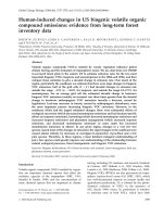
Abstract
Trends in the composition and reactivity of volatile organic compound (VOC) emissions from
motor vehicles are described over a 10-year period between 1991 and 2001. Vehicle emissions
were measured at the Caldecott tunnel in the San Francisco Bay area in summers 1991, 1994-97,
1999, and 2001. Concurrent liquid gasoline samples were collected from service stations in
Berkeley in summers 1995, 1996, 1999, and 2001. Fuel samples were also collected in
Sacramento during summer 2001 only. Gasoline headspace vapor composition was calculated
using the measured composition of liquid fuel samples and vapor-liquid equilibrium theory. As
a result of California’s reformulated gasoline (RFG) program, the reactivity of liquid gasoline
and headspace vapors were both reduced by ~20%, due mainly to lower aromatic and alkenes in
gasoline. The reactivity of tunnel non-methane organic compound (NMOC) emissions decreased
by 6% following the introduction of RFG, with reductions in C
9
+ aromatics being the most
important contributor to this change. Though the reduction in tunnel NMOC reactivity is likely
to be helpful, a more important effect through the 1990s has been the significant reduction in the
total mass of NMOC emitted by vehicles. After 1996 when Phase 2 RFG requirements first took
effect, some refiners began supplying low- or zero-oxygenate gasoline blends in the Bay area.

Gasoline samples collected in Sacramento confirm differences in the pattern of oxygenate use
between the Bay area and the Central Valley, where Federal RFG program requirements make
oxygenate use mandatory. Other related differences include less use of trimethylpentanes in
Sacramento vs. Bay area gasoline. In summer 2001, we found only one major gasoline brand
using ethanol as an oxygenate; increased reliance on ethanol has occurred since that time due to
the phase-out of methyl tert-butyl ether (MTBE) and other ethers in gasoline.
2




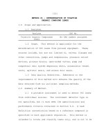
1. Introduction
Volatile organic compounds are important precursors to ozone and secondary particulate
matter, which affect both human health and global climate (Seinfeld and Pandis, 1997; IPCC,
2001). The main anthropogenic sources of volatile organic compounds are motor vehicle-related,
with significant additional emissions arising from solvent use in paints, consumer products, and
industrial processes (EPA, 1999). Natural VOC emissions from plants are also important.
Knowledge of the detailed chemical composition of VOC emissions from major source
categories is important because each individual VOC contributes differently to ozone and
secondary aerosol formation. VOC emission speciation is therefore an important input to source-
oriented photochemical models that are used to help design air pollution control strategies.
Exposure to some organic compounds also may pose human health hazards, and consequently
compounds such as benzene and 1,3-butadiene have been identified as hazardous air pollutants.
VOC composition profiles also are used in receptor-oriented studies that seek to back-
calculate the contributions of various source categories to VOC concentrations observed at
ambient air monitoring sites. Accurate VOC profiles for major sources such as motor vehicles
are essential to successful application of the chemical mass balance model (Watson, 1984; Lin
and Milford, 1994; Fujita et al., 1995; Gertler et al., 1996; Schauer et al., 2002). Many
applications of CMB models have focused on understanding sources of VOC with respect to the
ozone problem. There is also increasing interest in using these models to expand knowledge

regarding the role of different VOC in the formation of secondary organic aerosol (Watson et al.,
2001).
The speciation of VOC emitted from motor vehicles reflects the chemical composition of
the fuel consumed, with additional species formed and emitted as products of incomplete
3




combustion. These products of incomplete combustion depend on fuel composition (Kaiser et al.,
1991; Hoekman, 1992; Leppard et al., 1992; Schuetzle et al., 1994). In addition to tailpipe
emissions, VOC emissions from motor vehicles include various categories of evaporative
emissions such as resting losses, running losses which occur during vehicle operation due to
liquid and vapor leaks in the fuel system, diurnal emissions due to venting of vapors from the
fuel tank as ambient temperature rises over the course of the day, and hot soak emissions that
occur due to residual engine heat at the end of a trip after the engine has been shut down. Current
inventories indicate roughly equal contributions to total VOC emissions from tailpipe and
evaporative sources, while other analyses suggest that tailpipe emissions are dominant (Pierson
et al., 1999). Some evaporative emissions closely resemble the composition of liquid fuel, in
cases such as liquid leaks or liquid fuel spillage during refueling. In other cases, evaporative
VOC emissions are heavily enriched in the lightest most volatile compounds present in the liquid
fuel, as for example the vapors displaced from a vehicle fuel tank as it is filled with liquid fuel.
Haskew et al. (1999) studied running loss evaporative emissions and found that the composition
of the emitted VOC was best described as a 50-50 mix of liquid gasoline and headspace vapor
compositions.
The speciation of VOC emissions from on-road motor vehicles has been characterized in
numerous past studies through measurements in roadway tunnels (Lonneman et al., 1986;
Zielinska and Fung, 1994; McLaren et al., 1996; Sagebiel et al., 1996; Fraser et al., 1998;
Kirchstetter et al., 1999; Touaty and Bonsang, 2000; Harley et al., 2001). VOC emission
speciation also has been reported based on laboratory dynamometer testing of individual vehicles

(Sigsby et al., 1987; Hochhauser et al., 1992; Hoekman, 1992; Leppard et al., 1992; Ho and
Winer, 1998). The main advantage of laboratory measurements is the ability to control test
4




conditions including fuel properties, ambient temperature, air conditioner usage, and driving
patterns. On-road studies sacrifice some control of test conditions, but benefit from a much
larger sample of in-use vehicles than can be tested in the laboratory one vehicle at a time.
Whereas laboratory studies can isolate exhaust via direct sampling of tailpipe emissions, tunnel
measurements return a composite of tailpipe and running loss evaporative emissions.
During the 1990s, significant changes were made to California gasoline. In the first phase
of California’s Reformulated Gasoline (RFG) program, effective in 1992, lead was banned,
detergent additives were required, and fuel vapor pressure was reduced. Phase 2 of California’s
RFG program was implemented in the first half of 1996. Changes to gasoline included increased
oxygenate content; reduced contents of sulfur, alkenes, benzene, and other aromatics; reduced
vapor pressure, and reductions of mid-point (T
50
) and heavy-end (T
90
) distillation temperatures.
Most refiners met oxygenate requirements in 1996 through addition of MTBE to gasoline. Since
1996, refiners have exercised the option to develop alternative gasoline formulations with equal
emissions-reduction potential according to a predictive model (ARB, 1994). For example, some
refiners have reduced their use of oxygenates in gasoline sold in the San Francisco Bay area by
making additional reductions in fuel sulfur content and other changes. Due to Federal mandates
that apply in areas with serious ozone air pollution problems, use of oxygenates in gasoline is a
firm requirement in most of the rest of California including Sacramento and the San Joaquin
Valley. In recent years, both MTBE and ethanol have been used as gasoline oxygenates in

California. By the end of 2003, blending of MTBE and other ethers in California gasoline had
been banned, and refiners switched to ethanol as a fuel oxygenate where one was needed. A
summary of the evolution of Bay area gasoline properties since 1994 is provided in Table 1.
5




The overall objective of the present research is to describe the chemical composition and
reactivity of NMOC emissions from motor vehicles during the summer 2000 Central California
Ozone Study, and to describe changes that occurred between 1990 and 2000. Separate
composition profiles are sought for on-road vehicle emissions, unburned liquid gasoline, and
gasoline vapor emissions.

6

Table 1. Summary of San Francisco Bay area gasoline properties
a
(mean ± 1σ) during summers 1994-2001.

gasoline
property
1994
1995
1996
1997
1998
1999
2000
2001

RVP
b
(kPa)
(psi)
51 ± 1
7.4 ± 0.1
51 ± 1
7.4 ± 0.1
48 ± 1
7.0 ± 0.1
49 ± 1
7.1 ± 0.1
48 ± 1
7.0 ± 0.1
49 ± 1
7.1 ± 0.1
49 ± 1
7.0 ± 0.1
49 ± 1
7.0 ± 0.1
sulfur (ppmw)
131 ± 41
81 ± 36
16 ± 9
12 ± 11
16 ± 8
10 ± 8
9 ± 2
10 ± 4
oxygen (wt%)

0.5 ± 0.3
0.2 ± 0.2
2.0 ± 0.3
1.6 ± 0.6
1.6 ± 0.6
1.7 ± 0.6
1.8 ± 0.3
1.5 ± 0.9
MTBE
c
(vol%)
2.7 ± 1.7
1.0 ± 0.9
10.7 ± 1.7
8.2 ± 3.7
7.4 ± 4.3
8.0 ± 4.0
7.8 ± 4.3
5.9 ± 5.6
TAME
d
(vol%)
N/A
N/A
N/A
N/A
0.5 ± 0.8
0.1 ± 0.1
0.1 ± 0.8
0.2 ± 0.5

ethanol (vol%)
N/A
N/A
N/A
N/A
0.5 ± 1.6
0.7 ± 2.1
0.0 ± 0.0
0.5 ± 1.3
alkane (vol%)
57.4 ± 4.8
56.6 ± 5.1
62.6 ± 2.5
65.4 ± 3.7
64 ± 3
66 ± 5
63 ± 5
65 ± 4
alkene (vol%)
7.9 ± 4.4
8.8 ± 3.5
3.3 ± 0.9
3.4 ± 1.2
3.6 ± 1.2
3.2 ± 2.1
4.5 ± 1.8
4.3 ± 1.7
aromatic (vol%)
31.9 ± 2.1
33.7 ± 3.3

23.5 ± 1.4
22.7 ± 1.4
24 ± 2
22 ± 3
25 ± 3
24 ± 2
benzene (vol%)
1.6 ± 0.4
1.5 ± 0.4
0.4 ± 0.1
0.4 ± 0.1
0.51 ± 0.08
0.52 ± 0.08
0.55 ± 0.07
0.48 ± 0.06
T
50
(°C)
(°F)
101 ± 4
214 ± 8
103 ± 2
218 ± 4
93.8 ± 2.2
199 ± 4
93.3 ± 1.7
200 ± 3
93.3 ± 1.7
200 ± 3
93.3 ± 1.1

200 ± 2
94.7 ± 2.7
202 ± 5
94.4 ± 1.1
202 ± 2
T
90
(°C)
(°F)
168 ± 4
334 ± 8
172 ± 4
341 ± 8
149 ± 2
300 ± 4
148 ± 3
299 ± 6
151 ± 4
304 ± 8
152 ± 6
306 ± 10
151 ± 4
305 ± 7
149 ± 2
301 ± 3
density (g L
-1
)
761 ± 8
760 ± 4

743 ± 2
741 ± 5
746 ± 5
742 ± 6
742 ± 6
743 ± 7

a
Sales-weighted average of regular, mid-grade and premium gasoline. Service station samples collected during July in Concord and August in San Francisco,
and analyzed by Southwest Research Institute.
b
RVP is Reid Vapor Pressure.
c
MTBE is methyl tertiary butyl ether.
d
TAME is tert-amyl methyl ether.
7




2. Methods
2.1 Field Sampling
Vehicle emissions were measured in the Caldecott tunnel on highway 24 near Berkeley,
California. This tunnel has three bores with two lanes of traffic per bore, on a 4% grade. All
tunnel samples reported here were 2-hour averages collected in evacuated stainless steel canisters
on summer weekdays from 4-6 PM. In addition to the data of Zielinska and Fung (1994) and
Kirchstetter et al. (1999) for 1991 and 1994-97 presented previously, new data from 1999 and
2001 are presented here to permit analysis of emission trends over a 10-year period.
Measurements reported here represent emissions from a light-duty gasoline-powered vehicle

fleet operating in a warmed-up mode. The number of samples collected each year from 1994 to
2001 varied between 8 and 12.
In 1991, tunnel sampling took place on three afternoons, with 2 co-located samples
obtained on two of those days, and a single sample obtained on a third day, for a total of 5
samples (Zielinska and Fung, 1994). Samples in 1991 were collected in bore 1 of the tunnel, in
contrast to later measurements which were all obtained in bore 2, where heavy trucks are not
allowed. Note that even in bore 1, for 4-6 PM samples, the influence of diesel trucks is minimal
because they have relatively low VOC emission factors, and furthermore in the afternoon
commuter peak period, heavy trucks represent a small fraction of total traffic.
Tunnel concentrations were generally adjusted to account for background levels of
pollutants outside the tunnel. Background concentrations were not measured in 1991, so in
effect, zero concentration for all species at the entrance to the tunnel was assumed for the 1991
sampling. For 1994-1997, background concentrations were measured in fresh air that was being
injected by ventilation fans into the tunnel. In 1999 and 2001, background measurements were
8




made at the tunnel entrance with all ventilation fans turned off, allowing a complete mass
balance on air flowing through the tunnel. In the past, tunnel concentrations of emitted
hydrocarbons were typically much higher than background levels, so differences in handling of
background concentrations prior to 1999 are not likely to affect the results reported here.
To determine carbonyl (i.e., aldehyde and ketone) concentrations, additional tunnel and
background air samples were collected using dinitrophenylhydrazine (DNPH)-coated silica gel
cartridges over 2-h integrated sampling periods from 4 to 6 PM. These samples were co-located
with the hydrocarbon canister samples described above.
Liquid gasoline samples were collected at service stations during summer 2001 in
Berkeley and Sacramento, California. One liter each of regular and premium grade gasoline was
dispensed into separate steel cans for each of 5 major brands in each area. These samples provide

a snap-shot of how each refiner chose to meet applicable reformulated gasoline program
requirements. Similar samples of liquid gasoline were collected previously in Berkeley during
summers 1995, 1996, and 1999.
2.2 Analytical Methods
NMHC concentrations in tunnel canister samples were quantified using gas
chromatography with flame ionization detection, following generally similar procedures in all
years. Sampling procedures for 1991 and 1994-1997 are presented in detail elsewhere (Zielinska
and Fung, 1994; Kirchstetter et al., 1999). In 1991, a modified Chrompack Purge and Trap
Injector was used as the cryogenic trapping unit and a 50 m CP-Sil 5 CB capillary column was
used for separation. Samples for 1994-1996 were concentrated with a Nutech model 8548
cryogenic concentrator and injected into a Perkin-Elmer model 8500 GC outfitted with a 30 m
DB-1 column. For summers 1997, 1999, and 2001, samples were preconcentrated with a Nutech
9




model 3550A cryogenic concentrator and injected into a Varian CP-3800 gas chromatograph
equipped with a DB-1 capillary column. All speciated hydrocarbon analyses of tunnel air
samples were conducted by Hesson and coworkers at the Bay Area Air Quality Management
District’s laboratories in San Francisco, except for the 1991 data of Zielinska and Fung.
After eluting DNPH cartridge samples in acetonitrile, aldehyde and ketone concentrations
were quantified using high-performance liquid chromatography (HPLC) using a procedure very
similar to that described by Siegl et al. (1992). Carbonyls were quantified by Hoekman and
coworkers at Chevron for 1994-96, and by Fung in 1997. In more recent summers (i.e., 1999
and 2001), carbonyl concentrations were determined using a more detailed liquid
chromatographic technique with specialized detectors that allowed for quantification of many
more carbonyls in the tunnel air samples (Grosjean et al., 1999; Kean et al., 2001).
Detailed liquid gasoline speciation was determined for each gasoline sample by gas
chromatography on a Hewlett Packard Model 5890 II GC equipped with dual flame ionization

detectors. Primary analysis was performed on a DB-1 capillary column, with co-eluting peaks
resolved on a DB-5 column. These analyses were conducted by Kohler and coworkers at
ChevronTexaco in Richmond, CA. Typically ~300 species were identified in liquid gasoline
samples.
2.3 Headspace Vapor Composition
Headspace vapor composition was estimated in this study from the composition of liquid
gasoline using vapor-liquid equilibrium theory, as described previously by Kirchstetter et al.
(1999) assuming ideal solution behavior, and by Harley et al. (2000) for non-ideal ethanol-
gasoline mixtures. Briefly, measured liquid-phase mol fractions x
i
for each species present in
10




gasoline are multiplied by pure liquid vapor pressures

!
p
i
o
(T)
and activity coefficients
γ
i
to
estimate the partial pressure p
i
of each species in the vapor phase (eq 1).

!
p
i
=
"
i
x
i
p
i
o
(T)
(1)
Pure liquid vapor pressures are estimated using the Wagner equation as recommended by Reid et
al. (1987). In most cases, we assume
γ
i
=1 for all species present in liquid fuel (see Harley et al.
(2000) for values of
γ
i
when ethanol is present). Vapor phase mol fractions are computed as y
i
=
p
i
/ p
TOT
, where p

TOT
is simply the sum of all p
i
. Using the molecular weight of each species
present in the vapors, it is straightforward to convert from mol fraction y
i
to weight fraction w
i
in
the headspace vapors (eq 2).
!
w
i
=
y
i
M
i
y
i
M
i
i
"
(2)
The results when expressed in terms of relative composition are not very sensitive to
temperature; it is the absolute vapor pressure of gasoline that depends strongly on T, much
moreso than the relative composition of the vapors. We use conditions of a hot summer day (T =
38°C = 100°F) in the present analysis.
2.4 Reactivity of Emissions

The maximum incremental reactivity scale (MIR; Carter, 1994) is used to calculate the
normalized reactivity of NMOC emissions. MIR is defined under conditions where ozone
production is most sensitive to organic gas emissions. Current MIR values based on the
SAPRC99 chemical mechanism (Carter, 2002) are combined with NMOC emission profiles that
specify the weight fractions w
i
of each individual species to determine normalized reactivity R,
expressed as the incremental mass of O
3
produced per increment of NMOC mass emitted. As
absolute values of R are affected by various modeling assumptions and uncertainties, R is more
11




meaningful and robust when compared in a relative sense to similar values for other fuels and/or
years. The SAPRC99-based MIR values are generally higher than what we have used in
previous assessments of VOC reactivity (Kirchstetter et al., 1999).

3. Results and Discussion
3.1 Tunnel NMOC Emissions
Trends in the composition of non-methane organic compound (NMOC) emissions by
species class are presented in Figure 1. Effects of California Phase 1 reformulated gasoline use
after 1992 are hard to see, whereas the transition to Phase 2 RFG between 1995 and 1996 is
readily apparent. Between 1991 and 1994, the n-butane weight fraction in tunnel emissions
decreased from 3.4 ± 0.3% to 2.2 ± 0.2%, consistent with the targeted removal of C
4

hydrocarbons to achieve reductions in gasoline vapor pressure. Starting in 1996, there was a

large increase in MTBE emissions (listed as oxygenates in Figure 1), an increase in highly
branched alkanes, and a large reduction in aromatics. Isobutene and formaldehyde increased due
to increased use of MTBE in gasoline, though the change in isobutene is a small increment
compared to ethene and propene that dominate the alkene fraction shown in Figure 1. After 1996
there was a decrease in the mass fractions of both MTBE (5.8 ± 0.7% in 1996 versus 4.0 ± 0.5%
in 2001) and acetylene (4.9 ± 0.2% in 1996 versus 2.9 ± 0.6% in 2001); no other trends are
apparent in Figure 1 after 1996. Carbonyl reactivity is dominated by formaldehyde (see Kean et
al., 2001); overall carbonyls accounted for ~4 wt% of tunnel NMOC emissions. Note that
carbonyl data were not available for 1991.
12
Figure 1. Composition of tunnel non-methane organic compound emissions by class.
Figure 2. Normalized reactivity of tunnel emissions calculated using Carter’s MIR scale.
0%
20%
40%
60%
80%
100%
1991 1992 1993 1994 1995 1996 1997 1998 1999 2000 2001
wt %
n-alkanes
isoalkanes
cycloalkanes
alkenes
aromatics
acetylene
oxygenates
carbonyls
0
1

2
3
4
5
1991 1992 1993 1994 1995 1996 1997 1998 1999 2000 2001
normalized reactivity
13




Figure 2 shows that aromatics and alkenes are the dominant contributors to normalized
reactivity of tunnel NMOC emissions. Normalized reactivity values are higher than those
presented previously for 1994-1997 by Kirchstetter et al. (1999), due to upward revision of MIR
values by Carter (2002). In our current assessment, the use of Phase 2 RFG reduced the reactivity
of tunnel NMOC emissions by ~6%, due primarily to reduced levels of C
9
+
aromatics. This
reduction in reactivity is expected to be beneficial in terms of air quality, but is of lesser
importance compared to the reduction in NMOC mass emissions that occurred during the 1990s
as a combined result of California’s low-emission vehicle and reformulated gasoline programs
(see Kean et al., 2002).
Figure 3 focuses specifically on aromatic hydrocarbons present in tunnel emissions. The
reduction in fuel benzene and total aromatic contents required as part of Phase 2 RFG is clearly
apparent in Figure 3, with the benzene weight fraction in tunnel emissions dropping from 6.0 ±
0.3% in 1995 to 3.6-4.2% in 1996 and later years. To reduce the total aromatic content in phase 2
RFG, refiners also targeted C
9
and heavier aromatics. In contrast, C

8
aromatics (xylenes and
ethylbenzene) decreased only slightly between 1995 and 1996, and toluene showed no change.
Reducing heavy hydrocarbons such as C
9
+ aromatics was helpful in achieving a lower T
90

distillation temperature (Koehl et al., 1993). In contrast to benzene and monosubstituted
aromatics such as toluene and ethylbenzene, the C
9
+ aromatics consist mostly of di- and tri-
substituted aromatics that are highly reactive. For example, trimethylbenzenes are on average ~4
times more reactive than propylbenzene, which has the same molecular weight (Carter, 2002).
In our 2001 measurements at the Caldecott tunnel, a central research objective was to
study the effect of engine load on vehicle emissions. Therefore we measured emissions from 4-6
PM for moderate-load uphill driving on a 4% grade, and also in the morning at the same location
14
Figure 3. Aromatic hydrocarbons in tunnel emissions, as a fraction of total NMOC. C9+ includes highly reactive aromatics such as
ethyltoluene, diethylbenzene, and trimethylbenzene isomers.
0%
10%
20%
30%
40%
1991 1992 1993 1994 1995 1996 1997 1998 1999 2000 2001
wt %
Benzene Toluene m/p-Xylene o-Xylene Ethylbenzene C9+ Aromatics
15
Figure 4. Abundance of individual VOC in tunnel emissions for uphill vs downhill driving during summer 2001.

0%
2%
4%
6%
8%
10%
12%
0% 2% 4% 6% 8% 10% 12%
Downhill wt %
Uphill wt %
Toluene
Isopentane
m/p-Xylene
MTBE
2-Methylpentane
Ethene
Propene
Benzene
2,2,4-Trimethylpentane
16




with downhill driving and much lighter engine load. Interestingly, the absolute concentrations of
NMOC at the tunnel exit were almost as high for downhill as for uphill driving, while CO
2
was
much higher in uphill driving (see Kean et al., 2003). The relative composition of NMOC
emissions for uphill and downhill driving was generally similar, as shown in Figure 4. A

regression of individual species weight fractions plotted for uphill vs. downhill driving results in
a slope of 0.98 and R
2
= 0.95. The vast majority of species fell on or near the 1:1 line (see Figure
4). The relative abundances of ethene, propene, and benzene were higher in uphill driving,
consistent with formation of these species as combustion byproducts (Bailey et al., 1990; Ho and
Winer, 1998; Kirchstetter et al, 1999). In contrast, unburned fuel species such as 2-
methylpentane, 2,2,4-trimethylpentane, and methylcyclopentane, among others, were more
abundant in downhill emissions.
3.2 Liquid Gasoline
The measured compositions of liquid gasoline collected in Berkeley (summers 1995,
1996, 1999, and 2001) and Sacramento (summer 2001 only) are summarized in Figure 5. The
largest changes in fuel composition occurred between 1995 and 1996: both aromatics and
alkenes were reduced in liquid gasoline. Offsetting the decrease in aromatics between 1995 and
1996 were increases in MTBE and isoalkanes, especially highly branched alkanes such as 2,2,4-
trimethylpentane (this compound is used to define the 100 octane number rating). The aromatic
reduction was also seen in tunnel emissions as shown in Figures 1 and 2 and discussed
previously. The reason that reduced alkene content in liquid gasoline did not lead to large
changes in alkene emissions is that unburned fuel present in exhaust emissions is augmented by
combustion-derived C
2
-C
4
alkenes that did not change much as a result of RFG. After 1996,
there is a gradual reduction in the use of oxygenates in Bay Area gasoline, which resulted from
17

some refiners selling gasoline with little or no oxygenate. In contrast, the Sacramento fuel
samples all had at least 2 wt% oxygen in all cases, as required by Federal RFG mandates. Only
one brand of gasoline used ethanol as the oxygenate in summer 2001 for both Berkeley and
Sacramento. The across the board use of oxygenates in Sacramento led to other differences in
fuel composition compared to Berkeley. For example, there was less use of trimethylpentanes
and similar compounds in Sacramento gasoline (these are included with isoalkanes in Figure 5).
These compounds would not be as much needed in Sacramento gasoline where MTBE and
ethanol were used and served as high-octane blending components.
As shown in Figure 6, the normalized reactivity of liquid gasoline decreased by 20-25%
as a result of the introduction of Phase 2 RFG. Liquid fuel reactivity is dominated by aromatics,
though some additional reduction in reactivity resulted from alkene reductions that occurred
between 1995 and 1996. Though Sacramento and Berkeley fuels differ in terms of oxygenate
and alkylate use, the reactivity of liquid fuels (dominated by aromatics) is virtually identical.
3.3 Gasoline Headspace Vapors
Gasoline headspace vapors are greatly enriched in the lighter fuel constituents relative to
liquid gasoline. Isopentane alone accounts for about a third of headspace vapor mass. n-Butane
and n-Pentane are also abundant in headspace vapors, as are oxygenates such as MTBE or
ethanol. This short list of compounds (n-butane, n-pentane, isopentane, and MTBE/ethanol)
together are responsible for over 60% of headspace vapor mass. As shown in Figure 7, aromatics
account for a small fraction of headspace vapor mass (compare with Figure 5 where aromatics
are 30% of liquid fuel). The reactivity of headspace vapors shown in Figure 8 shows a reduction
of ~20% associated with the introduction of RFG. However in contrast to liquid gasoline where
aromatics were the main driver, it was the reduction in light alkenes that led to lower normalized
18




reactivity of headspace vapors. Just as aromatics and T
90

distillation temperature specifications
interacted to focus efforts on reducing heavy aromatics in gasoline, RVP limits together with
alkene specifications may have helped to promote targeted reduction of C
4
-C
5
alkenes that are
the most volatile alkenes present in gasoline.
19
Figure 5. Composition of non-methane organic compounds in liquid gasoline by class.
Figure 6. Normalized reactivity of liquid gasoline calculated using Carter’s MIR scale.
0
20
40
60
80
100
Berkeley
1995
Berkeley
1996
Berkeley
1999
Berkeley
2001
Sacramento
2001
wt %
n-alkanes
isoalkanes

cycloalkanes
alkenes/dienes
aromatics
oxygenates
unident.
0
1
2
3
4
5
Berkeley
1995
Berkeley
1996
Berkeley
1999
Berkeley
2001
Sacramento
2001
normalized reactivity
4.0
3.1
3.0
3.2
3.2
20
Figure 7. Abundance of major VOC classes in gasoline headspace vapors.
Figure 8. Normalized reactivity of headspace vapors calculated using Carter’s MIR scale.

0
20
40
60
80
100
Berkeley
1995
Berkeley
1996
Berkeley
1999
Berkeley
2001
Sacramento
2001
wt %
n-alkanes
isoalkanes
cycloalkanes
alkenes/dienes
aromatics
oxygenates
0.0
0.5
1.0
1.5
2.0
2.5
3.0

Berkeley
1995
Berkeley
1996
Berkeley
1999
Berkeley
2001
Sacramento
2001
normalized reactivity
2.5
2.0
1.9
2.1
2.0
21




4. Conclusions
The chemical composition of gasoline and of vehicle NMOC emissions changed
significantly during the 1990s, mainly as a result of California’s reformulated gasoline program.
Noteworthy changes include reductions in C
4
-C
5
alkenes, benzene, and C
9

+ aromatics. At the
same time use of trimethylpentanes and oxygenates such as MTBE increased. While the
normalized reactivity of liquid gasoline and headspace vapors decreased by ~20%, the reactivity
of tunnel emissions decreased by only 6%. The smaller change in reactivity for tunnel emissions
is due to the presence in exhaust of reactive alkenes and aldehydes that were absent or only
minimally present in unburned fuel.
Between 1996 and 2000, the main change seen in Bay area gasoline was increased use of
low- or zero-oxygenate fuel blends by some refiners. Unlike the Bay area, use of oxygenates in
gasoline is a firm requirement in the Central Valley of California. Sacramento gasoline samples
collected in summer 2001 indicate across the board use of oxygenates in all brands and grades of
gasoline. Differences in patterns of oxygenate use between the Bay area and Sacramento led to
other fuel differences such as less use of trimethylpentanes in Sacramento gasoline. In summer
2001, only one major brand of gasoline sold in Central California used ethanol as a fuel
oxygenate.
22




5. Recommendations
As California gasoline was reformulated early in 1996, we recommend speciation profiles
based on summer 1996 and later data only for use with the summer 2000 Central California
Ozone Study. Of the profiles reported here, the summer 1999 and 2001 fuel and tunnel profiles
are close matches for the Bay area in summer 2000.
Due to differences in the patterns of oxygenate use in gasoline sold in Central California,
different VOC speciation profiles are appropriate for vehicle emissions in the Bay area vs. the
Central Valley. Differences are likely to be largest for MTBE and trimethylpentanes. It will be
essential to capture regional differences in motor vehicle emission profiles in receptor modeling
studies that use those compounds as tracers. Due to its limited use as a fuel oxygenate prior to
2003, ethanol is not appropriate as a tracer for vehicle-related emissions in summer 2000. In

photochemical modeling studies, the differences in normalized reactivity of various emission
profiles measured since 1996 appear to be small, and could probably be neglected because the
mass of VOC emissions has a greater impact on photochemical model O
3
predictions than
relatively subtle differences in VOC composition.
To address uncertainties in the relative importance of tailpipe vs. evaporative sources of
vehicle emissions, we recommend reconciliation of source profiles presented here with time-
resolved ambient VOC concentration measurements made during CCOS.
23




Literature Cited
ARB (1994). Proposed amendments to the California Phase 2 reformulated gasoline regulations,
including amendments for the use of a predictive model. California Air Resources Board,
Sacramento, CA.

Bailey, J., Schmidl, B., Williams, M. (1990). Speciated hydrocarbon emissions from vehicles
operated over the normal driving speed range on the road. Atmospheric Environment 24A, 43-52.

Carter, W.P.L. (1994). Development of ozone reactivity scales for volatile organic compounds.
Journal of the Air & Waste Management Association 44, 881-899.

Carter, W.P.L. (2002). VOC Reactivity Data.
accessed November 2002. University of California, Riverside, CA.

EPA (1999). National Air Quality and Emissions Trends Report. U.S. Environmental Protection
Agency, Office of Air Quality Planning and Standards, Research Triangle Park, NC.

Fraser, M.P., Cass, G.R., Simoneit, B.R.T. (1998). Gas-phase and particle-phase organic
compounds emitted from motor vehicle traffic in a Los Angeles roadway tunnel. Environmental
Science & Technology, 32, 2051-2060.

Fujita, E.M., Watson, J.G., Chow, J.C. (1995). Receptor model and emission inventory source
apportionments of nonmethane organic gases in California’s San Joaquin Valley and San
Francisco Bay Area. Atmospheric Environment 29, 3019-3035.

Gary, J.H., Handwerk, G.E. (2001). Petroleum refining: technology and economics, 4
th
Edition.
Marcel Dekker, New York.

Gertler, A.W., Fujita, E.M., Pierson, W.R., Wittorff, D.N. (1996). Apportionment of NMHC
tailpipe and non-tailpipe emissions in the Fort McHenry and Tuscarora Mountain tunnels.
Atmospheric Environment 30, 2297-2305.

Gorse, Jr., R.A., Benson, J.D., Burns, V.R., Hochhauser, A.M., Koehl, W.J., Painter, L.J.,
Reuter, R.M., Rippon, B.H. (1991). Toxic air pollutant vehicle exhaust emissions with
reformulated gasolines. SAE Technical Paper Series no. 912324.

Grosjean, E.; Green, P.G.; Grosjean, D. (1999). Liquid chromatography analysis of carbonyl
(2,4-dinitrophenyl)hydrazones with detection by diode array ultraviolet spectroscopy and by
atmospheric pressure negative chemical ionization mass spectrometry. Analytical Chemistry 71,
1851-1861.

Harley, R.A., Sawyer, R.F., Milford, J.B. (1997). Updated photochemical modeling for
California’s South Coast Air Basin: Comparison of chemical mechanisms and motor vehicle
emission inventories. Environmental Science & Technology 31, 2829-2839.

24