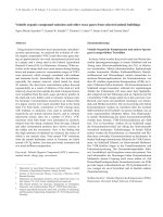
Atmospheric volatile organic compound measurements during the Pittsburgh Air Quality Study: Results, interpretation, and quantification of primary and secondary contributions pot
Bạn đang xem bản rút gọn của tài liệu. Xem và tải ngay bản đầy đủ của tài liệu tại đây (577.66 KB, 17 trang )
Atmospheric volatile organic compound measurements during
the Pittsburgh Air Quality Study: Results, interpretation, and
quantification of primary and secondary contributions
Dylan B. Millet,
1,2
Neil M. Donahue,
3
Spyros N. Pandis,
3
Andrea Polidori,
4
Charles O. Stanier,
2,5
Barbara J. Turpin,
4
and Allen H. Goldstein
1
Received 3 February 2004; revised 7 April 2004; accepted 22 April 2004; published 25 January 2005.
[1] Primary and secondary contributions to ambient levels of volatile organic compounds
(VOCs) and aerosol organic carbon (OC) are determined using measurements at the
Pittsburgh Air Quality Study (PAQS) during January–February and July–August 2002.
Primary emission ratios for gas and aerosol species are defined by correlation with
species of known origin, and contributions from primary and secondary/biogenic sources
and from the regional background are then determined. Primary anthropogenic
contributions to ambient levels of acetone, methylethylketone, and acetaldehyde were
found to be 12–23% in winter and 2–10% in summer. Secondary production plus
biogenic emissions accounted for 12–27% of the total mixing ratios for these compounds
in winter and 26–34% in summer, with background concentrations accounting for the
remainder. Using the same method, we determined that on average 16% of aerosol OC
was secondary in origin during winter versus 37% during summer. Factor analysis of the
VOC and aerosol data is used to define the dominant source types in the region for both
seasons. Local automotive emissions were the strongest contributor to changes in
atmospheric VOC concentrations; however, they did not significantly impact the aerosol
species included in the factor analysis. We conclude that longer-range transport and
industrial emissions were more important sources of aerosol during the study period. The
VOC data are also used to characterize the photochemical state of the atmosphere in the
region. The total measured OH loss rate was dominated by nonmethane hydrocarbons
and CO (76% of the total) in winter and by isoprene, its oxidation products, and
oxygenated VOCs (79% of the total) in summer, when production of secondary organic
aerosol was highest.
Citation: Millet, D. B., N. M. Donahue, S. N. Pandis, A. Polidori, C. O. Stanier, B. J. Turpin, and A. H. Goldstein (2005),
Atmospheric volatile organic compound measurements during the Pittsburgh Air Quality Study: Results, interpretation, and
quantification of primary and secondary contributions, J. Geophys. Res., 110, D07S07, doi:10.1029/2004JD004601.
1. Introduction
[2] Airborne particulate matter (PM) can adversely affect
human and ecosystem health, and exerts considerable
influence on climate. Effective PM control strategies require
an understanding of the processes controlling PM concen-
tration and composition in different environments. The
Pittsburgh Air Quality Study (PAQS) is a comprehensive,
multidisciplinary project directed at understanding the pro-
cesses governing aerosol concentrations in the Pittsburgh
region [e.g., Wittig et al., 2004a; Stanier et al., 2004a,
2004b]. Specific objectives include characterizing the phys-
ical and chemical properties of regional PM, its morphology
and temporal and spatial variability, and quantifying the
impacts of the important sources in the area.
[
3] Volatile organic compounds (VOCs) can directly
influence aerosol formation and growth via condensation
of semivolatil e oxidation products onto existing aerosol
surface area [Odum et al., 1996; Jang et al., 2002; Czoschke
et al., 2003], and possibly via the homogeneous nucleation
of new particles [Koch et al., 2000; Hoffmann et al., 1998].
They also have strong indirect effects on aerosol via their
control over ozone production and HO
x
cycling, which in
turn dictate oxidation rates of organic and inorganic aerosol
precursor species. Comprehensive and high time resolution
VOC measurements in conjunction with particle measure-
ments thus aid in characterizing chemical conditions con-
JOURNAL OF GEOPHYSICAL RESEARCH, VOL. 110, D07S07, doi:10.1029/2004JD004601, 2005
1
Division of Ecosystem Sciences, University of California, Berkeley,
California, USA.
2
Now at Depa rtment of Earth and Planetary Sciences, Harvard
University, Cambridge, Massachusetts, USA.
3
Department of Chemical Engineering, Carnegie Mellon University,
Pittsburgh, Pennsylvania, USA.
4
Department of Environmental Sciences, Rutgers University, New
Brunswick, New Jersey, USA.
5
Now at Department of Chemical and Biochemical Engineering,
University of Iowa, Iowa City, Iowa,USA.
Copyright 2005 by the American Geophysical Union.
0148-0227/05/2004JD004601$09.00
D07S07 1of17
ducive to particle formation and growth. VOC data can also
yield information on the nature of source types impacting
the study region [Goldstein and Schade, 2000], photochem-
ical aging and transport phenomena [Parrish et al., 1992;
McKeen and Liu, 1993], and estimates of regional emission
rates [Barnes et al., 2003; Bakwin et al., 1997], all of which
can be useful in interpreting other gas and particle phase
measurements.
[
4] This paper describes the results from two field deploy-
ments, during January–February 2002 and July –August
2002, in which we made in situ VOC measurements along-
side the comprehensive aerosol measurements at the PAQS
site, with the aim of specifically addressing the connection
between atmospheric trace gases and particle formation and
source attribution. The data set provides an opportunity to
examine aerosol formation and chemistry in the context of
high time resolution speciated VOC measurements.
[
5] The specific goals of this paper include: characteriz-
ing the dominant source types impacting the Pittsburgh
region, their composition and variability; assessing the
relative importance of different types of VOCs to regional
photochemistry, and the relationship between aerosol con-
centrations and the chemical state of the atmosphere; and
quantifying the relative importance of primary and second-
ary sources in determining organic aerosol and oxygenated
VOC (OVOC) concentrations. For the latter we quantify the
primary emission ratios for species with multiple source
types, by correlation with combustion and photochemical
marker compounds.
2. Experimental
2.1. Pittsburgh Air Quality Study (PAQS)
[
6] The field component of the Pittsburgh Air Quality
Study was carried out from July 2001 through August 2002 .
Measurement platforms consisted of a main sampling site
located in a park about 6 km east of downtown Pittsburgh,
as well as a set of satellite sites in the surrounding region.
For details on the PAQS study, see Wittig et al. [2004a] and
the references cited therein. Measurements described here
were made at the main sampling site.
2.2. VOC Measurements
[
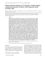
7] A schematic of the VOC measurement setup is shown
in Figure 1. To provide information on as wide a range of
compounds as possible, two separate measurement channels
were used, equipped with different preconditioning systems,
preconcentration traps, chromatography columns, and
detectors. Channel 1 was designed for preconcentration
and separation of C
3
–C
6
nonmethane hydrocarbons, includ-
ing alkanes, alkenes and alkynes, on an Rt-Alumina PLOT
column with subsequent detection by FID. Channel 2 was
designed for preconcentration and separation of oxygenated,
aromatic, and halogenated VOCs, NMHCs larger than C
6
,
and some other VOCs such as acetonitrile and dimethylsul-
fide, on a DB-WAX column with subsequent detection by
quadropole MSD (HP 5971).
[
8 ] Air samples were d rawn at 4 s l/min through a
2 micron Teflon particulate filter and 1/4
00
OD Teflon tubing
(FEP fluoropolymer, Chemfluor) mounted on top of the
laboratory container. Two 15 scc/min subsample flows were
drawn from the main sample line, and through pretreatment
traps for removal of O
3
,H
2
O and CO
2
. For 30 min out of
every hour, the valve array (V1, V2, and V3; valves from
Valco Instruments) was switched to sampling mode
(Figure 1, as shown) and the subsamples flowed through
0.03
00
ID fused silica-lined stainless steel tubing (Silcosteel,
Restek Corp) to the sample preconcentration traps where
the VOCs were trapped prior to analysis. When sample
collection was complete, the preconcentration traps and
downstream tubing were purged with a forward flow of
UHP helium for 30 s to remove residual air. The valve array
was then switched to inject mode, the preconcentration traps
heated rapidly to 200°C, and the trapped analytes desorbed
into the helium carrier gas and transported to the GC for
separation and quantification.
Figure 1. Schematic of the VOC sampling system. MFC, mass-flow controller; V1–V3, valves 1–3;
MSD, mass selective detector; FID, flame ionization detector; PT, pressure transducer.
D07S07 MILLET ET AL.: VOLATILE ORGANICS AT THE PITTSBURGH SUPERSITE
2of17
D07S07
[9] As noninert surfaces are known to cause artifacts and
compound losses for unsaturated and oxygenated species,
all surfaces contacted by the sampled airstream prior to the
valve array were constructed of Teflon (PFA or FEP). All
subsequent tubing and fittings, except the internal surfaces
of the Valco valves V1, V2, and V3, were Silcosteel. The
valve array, including all silcosteel tubing, was housed in a
temperature controlled box held at 50°C to prevent com-
pound losses through condensation and adsorption. All
flows were controlled using Mass-Flo Controllers (MKS
Instruments), and pressures were monitored at various
points in the sampling apparatus using pressure transducers
(Data Instruments).
[
10] In order to reduce the dew point of the sampled
airstream, both subsample flows passed through a loop of
1/8
00
OD Teflon tubing cooled thermoelectrically to À25°C.
Following sample collection, the water trap was heated to
105°C while being purged with a reverse flow of dry zero
air to expel the condensed water prior to the next sampling
interval. A trap for the removal of carbon dioxide and
ozone (Ascarite II, Thomas Scientific) was placed down-
stream of the water trap in the Rt-Alumina/FID channel.
An ozone trap (KI-impregnated glass wool, following
Greenberg et al. [1994]) was placed upstream of the water
trap in the other channel leading to the DB-WAX column
and the MSD (Figure 1).
[
11] Sample preconcentration was achieved using a com-
bination of thermoelectric cooling and adsorbent trapping.
The preconcentration traps consisted of three stages (glass
beads/Carbopack B/Carboxen 1000 for the Rt-Alumina/FID
channel, glass beads/Carbopack B/Carbosieves SIII for the
DB-WAX/MSD channel; all adsorbents from Supelco), held
in place by DMCS-treated glass wool (Alltech Associates)
in a 9 cm long, 0.04
00
ID fused silica-lined stainless steel
tube (Restek Corp). A nichrome wire heater was wrapped
around the preconcentration traps, and the trap/heater
assemblies were housed in a machined aluminum block
that was thermoelectrically cooled to À15°C. After sample
collection and the helium purge, the preconcentration traps
were isolated via V3 (see Figure 1) until the start of the next
chromatographic run. The traps were small enough to
permit rapid thermal desorption (À15°C to 200°Cin10s)
eliminating the need to cryofocus the samples before chro-
matographic analysis (following Lamanna and Goldstein
[1999]). The samples were thus introduced to the individual
GC columns, where the components were separated and
then detected with the FID or MSD.
[
12] Chromatographic separation and detection of the
analytes was achieved using an HP 5890 Series II GC.
The temperature program for the GC oven was: 35°Cfor
5min,3°C/min to 95°C, 12.5°C/min to 195°C, hold for
6 min. The oven then ramped down to 35°C in preparation
for the next run. The carrier gas flow into the MSD
was controlled electronically and mai ntained constant at
1 mL/min. The FID channel carrier gas flow was controlled
mechanically by setting the pressure at the column head
such that the flow was 4.5 mL/min at an oven temperature
of 35°C. The carrier gas for both channels was UHP
(99.999%) helium which was further purified of oxygen,
moisture and hydrocarbons (traps from Restek Corp.).
[
13] Zero air for blank runs and calibration by standard
addition was generated by flowing ambient air over a bed of
platinum heated to 370°C. This system passes ambient
humidity, creating VOC free air in a matrix resembling real
air as closely as possible. Zero air was analyzed daily to
check for blank problems and contamination for all mea-
sured compounds.
[
14] Compounds measured on the FID channel were
quantified by determining their weighted response relative
to a reference compound (see Goldstein et al. [1995a] and
Lamanna and Goldstein [1999] for details). Neohexane
(5.15 ppm, certified NIST traceable ±2%; Scott-Marrin
Inc.) was employed as the internal standard for the FID
channel, and was added by dynamic dilution to the sam-
pling stream. Compound identification was achieved by
matching retention times with those of known standards
for each compound (Scott Specialty Gases, Inc.).
[
15] The MSD was operated in single ion mode (SIM) for
optimum sensitivity and selectivity of response. Ion-
monitoring windows were timed to coincide with the elution
of the compounds of interest. Calibration curves for all of
the individual compounds were obtained by dynamic dilu-
tion of multicomponent low-ppm level standards (Apel-
Riemer Environmental Inc.) into zero air to mimic the range
of ambient mixing ratios. A calibration or blank was
performed every 6th run.
[
16] The system was fully automated for unattended
operation in the field. The valve array (V1, V2 and V3)
and the preconcentration trap resistance heater circuit were
controlled through the GC via auxiliary output circuitry. The
PC controlling the GC was also interfaced with a CR10X
data logger (Campbell Scientific Inc.), which was triggered
at the outset of each analysis run. The inlet valve, the
standard addition solenoid valve and the water trap cooling,
heating and valve circuitry were switched at the appropriate
times during the sampling cycle by a relay module (SDM-
CD16AC, Campbell Scientific) controlled by the data
logger. Relevant engineering data (time, temperatures, flow
rates, pressures, etc.) for each sampling interval were
recorded by the CR10X data logger with a AM416 multi-
plexer (Campbell Scientific Inc.), then uploaded to the PC
and stored with the associated chromatographic data. Chro-
matogram integrations were done using HP Chemst ation
software. All subsequent data processing and QA/QC
was performed using routines created in S-Plus (Insightful
Corp.). Instrumental precision, detection limits, and
accuracy for each measured compound during this experi-
ment, along with the 0.25, 0.50, and 0.75 quantiles of the
data, are given in Table 1.
2.3. Aerosol, Trace Gas, and Meteorological
Measurements
[
17] Additional measurements which are used in this
paper are described briefly below. For a more thorough
overview of the gas and particle measurement methods and
results from PAQS, the reader is directed to Wittig et al.
[2004a] and the references cited therein.
[
18] Semicontinuous measurements of PM 2.5 (i.e.,
<2.5 mm diamete r) particulate mass were made using a
tapering element oscillating microprobe (TEOM) instrument
(Model 1400a, Rupprecht & Patashnick Co., Inc.). PM 2.5
nitrate and sulfate were also measured on a semicontinuous
basis using Integrated Collection and Vaporiz ation Cell
(ICVC) instruments (Rupprecht & Patashnick Co., Inc.)
D07S07 MILLET ET AL.: VOLATILE ORGANICS AT THE PITTSBURGH SUPERSITE
3of17
D07S07
[Wittig et al., 2004b]. Aerosol number size distributions
(0.003–10 mm) were quantified using an array of particle
sizing measurements: a nano scanning mobility particle sizer
(SMPS) (TSI, Inc., Model 3936N25), standard SMPS (TSI,
Inc., Model 3936L10), and Aerodynamic Particle Sizer
(APS) (TSI, Inc., Model 3320). Aerosol number size distri-
bution measurements were made semicontinuously through-
out the PAQS campaign [Stanier et al., 2004a]. Aerosol
organic carbon (OC) and elemental c arbon (EC) were
quantified in situ throughout the study with 2–4 hour time
resolution using a Sunset Labs in situ carbon analyzer
(A. Polidori et al., manuscript in preparation, 2005).
[
19]O
3
, NO, NO
2
, CO and SO
2
were measured contin-
uously with commercial gas analyz ers (Models 400A,
200A, 300 and 100A, Teledyne Advanced Pollution Instru-
mentation). Measurements of relevant meteorological
parameters (incoming radiation, air temperature, wind speed
and direction, precipitation, and relative humidity) were also
made continuously throughout the experiment.
3. Results and Discussion
3.1. Meteorological Conditions
[
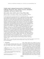
20] Observed wind speed and direction for the two study
periods (9 January to 12 February and 9 July to 10 August
2002) are shown as a wind rose plot in Figure 2. Through-
out this paper, data collected during the January–February
2002 deployment will be referred to as ‘‘winter’’ data and
Table 1. Concentration Quantiles and Figures of Merit for Measured VOCs
Compound
Precision,
a
%
Detection
Limit, ppt
Accuracy,
%
Winter
b
Summer
c
Median, ppt IQR,
d
ppt Median, ppt IQR,
d
Propane 2.5 1.6 7.6 2960 2087 – 4307 1787 992 – 3540
Isobutane 2.5 1.2 7.6 668 479–953 323 212 – 634
Butane 2.5 1.2 7.6 1333 978–1799 632 375 – 1106
Isopentane 2.5 0.9 7.6 575 448–809 649 409 – 1139
Pentane 2.5 0.9 7.6 355 279–493 352 213 – 613
Methylpentanes
e
2.5 0.8 7.6 268 203–368 276 183 – 506
Hexane 2.5 0.8 7.6 147 116–199 129 81–231
Propene 2.5 1.5 7.6 214 147–306 219 159 – 336
t-2-butene 2.5 1.1 7.6 30 19 –52 11 8 –18
1-butene 2.5 1.1 7.6 57 40 –83 62 44 –88
2-methylpropene 2.5 1.1 7.6 38 32 –51 NQ
f
NQ
f
Cyclopentane 2.5 0.9 7.6 53 35 –92 47 36 –72
c-2-butene 2.5 1.1 7.6 27 18 –44 20 15 –28
Cyclopentene 2.5 1.0 7.6 NQ
f
NQ
f
30–8
Propyne 2.5 1.4 7.6 29 22 –40 7 5–12
3-methyl-1-butene 2.5 0.9 7.6 6 5 –10 19 12 –35
t-2-pentene 2.5 0.9 7.6 19 12 –33 44 33 –62
1-pentene 2.5 0.9 7.6 36 24–56 20 14–32
2-methyl-1-butene 2.5 0.9 7.6 16 11 –25 42 22 –74
Benzene 4.4 26 10 279 231–355 215 143–405
Perchloroethylene 5.4 0.6 10 18 12– 25 22 13 – 41
Ethylbenzene 5.8 1.6 10 47 34–69 71 44 – 141
Isoprene 4.3 3.1 10 <DL
g
<DL
g
619 153 – 1475
Methyl-t-butyl ether 4.2 1.7 10 10 7 –14 31 19 –61
Acetaldehyde 7.2 82 10 538 403 –729 1559 1103 – 2150
Dimethylsulfide 5.6 3.2 10 NQ
f
NQ
f
75–10
Acetone 4.0 47 10 943 655 – 1385 4031 3128 – 4894
Butanal 6.0 28 10 NQ
f
NQ
f
91 64 –122
Methacrolein 5.6 11 10 <DL
g
<DL
g
266 178 – 366
3-methylfuran 4.2 2.2 10 <DL
g
<DL
g
10 6 –16
Methanol 8.2 370 11 3760 2347–5773 10717 7122 – 14601
Methylethylketone 5.1 10 10 215 153 –299 559 408 – 674
Methylene chloride 7.1 22 10 NQ
f
NQ
f
79 48 –145
Isopropanol 8.9 23 11 131 86– 199 235 147 – 432
Ethanol 13 16 15 989 673 –1416 1722 1017 – 3567
Methylvinylketone 3.5 6.8 10 <DL
g
<DL
g
463 273 – 665
Pentanal 8.3 19 11 NQ
f
NQ
f
137 98–193
Acetonitrile 13 38 14 NQ
f
NQ
f
131 105 – 155
Chloroform 3.6 1.2 10 11 10 – 13 17 13 – 30
a-pinene 5.9 0.6 10 <DL
g
<DL
g
16 10–29
Toluene 2.9 22 10 331 248 – 494 443 274 – 902
Hexanal 11 25 13 34 22 – 52 NQ
f
NQ
f
p-xylene 5.8 3.4 10 62 42 – 95 91 51 – 173
m-xylene 5.8 5.3 10 113 76 –176 163 89–306
o-xylene 5.8 2.4 10 60 41 – 89 52 29 – 93
a
Defined as the relative standard deviation of the calibration fit residuals.
b
Dates of 9 January to 12 February 2002.
c
Dates of 9 July to 10 August 2002.
d
IQR, interquartile range.
e
The sum of 2-methylpentane and 3-methylpentane, which coelute.
f
NQ, not quantified, due to inadequate resolution, unavailability of standard or other reason.
g
<DL, below detection limit.
D07S07 MILLET ET AL.: VOLATILE ORGANICS AT THE PITTSBURGH SUPERSITE
4of17
D07S07
that collected during July – August 2002 as ‘‘summer’’ data.
Winds in the winter were predominantly out of the west
(south to northwest), whereas in the summer southeasterly
and northwesterly winds were most common (Figure 2).
There was a diurnal cycle in wind speed in both seasons,
with stronger winds during the day and weaker winds at
night (not shown).
3.2. Factor Analysis
[
21] Factor analysis can be used to categorize measured
compounds into distinct source groups based on the covari-
ance of their concentrations, creating an understanding of
the variety of sources contributing to a broad range of
measured species [Sweet and Vermette, 1992; Thunis and
Cuvelier, 2000; Lamanna and Goldstein, 1999]. In this
section we characterize the dominant source types impact-
ing the Pittsburgh region in summer and winter, based on a
factor analysis of the VOC data set, combined with other
available trace gas and high temporal resolution aerosol
data. Compounds are grouped into factors according to their
covariance, and the strength of association between com-
pounds and factors is expressed as a loading matrix. Each
factor is a linear combination of the observed variables and
in theory represents an underlying process which is causing
certain species to behave similarly. Prior knowledge of
source types for the dominant compounds is then used to
assign source categories to the statistically identified factors.
[
22] The analysis was performed using principal compo-
nents extraction and varimax rotation (S-Plus 6.1, Lucent
Technologies Inc.). Species having a significant amount
(>8%) of missing data were excluded from the analysis.
Results for the winter and summer data sets are presented in
Tables 2 and 3, respectively, and discussed in detail below.
Compounds not loading significantly on any of the factors
are omitted from the loadings tables.
3.2.1. Winter Trace Gas and Aerosol Data Set
[
23] Six factors were extracted from the winter data set,
which accounted for a total of 83% of the cumul ative
variance (Table 2). Each of the six factors accounted for a
statistically significant portion of the variance (P < 0.01,
where P is the statistical probability of incorrectly attribut-
ing a nonzero fraction of the variance to a given factor). The
analysis was limited to six factors since including more
factors failed to account for more than an additional 2% of
the variance in the data set.
[
24] Factor 1, explaining 44% of the total variability in
the data set, was associated most strongly with short-lived
combustion-derived pollutants, such as the anthropogenic
alkenes and aromatic species, in addition to NO
x
and the
gasoline additive methyl-t-butyl ether (MTBE). We attribute
this factor to local automobile emissions. The diurnal cycle
exhibited by this factor (Figure 3a) showed a clear pattern,
higher during the day than at night, and with prominent
peaks during the morning and evening rush hours. Note that
factor 1 accounted for 44% of the data set variability,
indicating that automobile exhaust was most strongly re-
sponsible for changes in atmospheric VOC concentrations
in Pittsburgh in the winter. Note also, however, that none of
the aerosol parameters included in the factor analysis (PM
2.5 mass, aerosol sulfate and nitrate mass, and aerosol
number density) loaded significantly on this factor, suggest-
ing that this source was a relatively minor contributor to
these components of regional PM.
[
25] Factor 2, accounting for 10% of the variance, was
associated exclusively with the anthropogenic alkanes
(Table 2), most strongly with propane, and probably repre-
sents leaks of propane fuel or natural gas. None of the
aerosol measurements loaded on this factor. Factor 2 was on
average highest with winds out of the south, and the diurnal
pattern showed a maximum in the early morning before
dawn (Figure 3b), with a minimum in the afternoon.
[
26] The third factor, accounting for 9% of the data set
variance, like factor 1 was associated with some gas-phase
combustion products (such as CO, benzene and propyne).
Unlike factor 1, however, it also contained a significant
aerosol component, in particular sulfate and PM 2.5 mass.
The diurnal cycle of factor 3 (Figure 3c) was distinct from
that of factor 1, with higher concentrations at night, and no
noticeable rush hour contribution. The highest levels of
factor 3 were seen with winds out of the south-southeast.
We attribute this factor to industrial emissions from point
sources in the region. In particular, the U.S. Steel Clairton
Works, which is the largest manufacturer of coke and coal
chemicals in the United States, and is located 11 miles to the
south-southeast of Pittsburgh, may have been a significant
contributor to this factor.
[
27] Factor 4 was composed of species (acetone, acetal-
dehyde, methylethylketone (MEK)) that are both emitted
directly and produced photochemicall y. Acetone and acet-
aldehyde are also known to have significant biogenic
sources [Schade and Goldstein, 2001]; however, biogenic
emissions are unlikely to be a dominant source of these
compounds in the Pittsburgh winter. PM 2.5 mass was also
associated with this category, consistent with the importance
of both primary emissions and secondary production of
regional aerosol. The diurnal cycle of factor 4 (Figure 3d)
showed evidence of both primary and secondary influence.
Daytime concentrations were slightly higher than at night,
and there was a marked increase in the morning which was
coincident with sunrise. Unlike factor 1, this factor did not
show the distinct morning and evening peaks coinciding
with rush hour. The day-night difference was much less than
in summer (see following section), likely reflecting weak
wintertime photochemistry and a consequently greater rel-
ative impact from direct emissions. The relative importance
of primary and photochemical sources for these compounds
is explored further in section 3.3.
[
28] Factor 5, which explained a further 6% of the
variance, was negatively associated with ozone and nuclei
mode aerosol number density, and positively associated
with total PM 2.5 mass, aerosol nitrate and accumulation
Figure 2. Wind rose plots for the winter and summer
experiments. The lengths of the wedges are proportional to
the frequency of observation.
D07S07 MILLET ET AL.: VOLATILE ORGANICS AT THE PITTSBURGH SUPERSITE
5of17
D07S07
mode number density. This factor may represent the com-
bined influences of photochemical activity and mixed layer
dynamics. Production of ozone and nucleation mode par-
ticles is driven by sunlight, and owing to their relatively
short lifetimes their concentrations were highest during the
day and lower at night. By contrast, l onger lived pollutants
less strongly impacted by photochemistry exhibited higher
concentrations at night when winds were calmer and verti-
cal mixing limited. In addition, partitioning of semivolatile
species such as nitrate into the particle phase is thermody-
namically favored by the colder temperatures and higher
relative humidity at night.
[
29] The 6th factor, accounting for 6% of the variability,
was associated with gas phase SO
2
, aerosol sulfate, PM 2.5
mass, and accumulation mode number density. Factor 6
showed a diurnal pattern with higher impact during the day
than at night, consistent with a photochemically driven
process (Figure 3f). However, nucleation mode number
density did not load significantly on this factor. This factor
may reflect regional coal burning power plant emissions of
gases and particles, and the subsequent pho tochem ical
aging of those emissions.
3.2.2. Summer Trace Gas and Aerosol Data Set
[
30] Six factors were extracted from the summer data set,
which together accounted for 77% of the variability in the
observations (Table 3). Each of the six factors accounted for
a statistically significant portion of the variance (P < 0.01).
Including additional factors explained less than 2% of the
remaining variance. The PM 2.5 measurements had a large
number (19%) of missing values, and as there was a strong
correlation (r
2
= 0.92) between PM 2.5 mass and aerosol
volume measured with the SMPS, missing PM 2.5 concen-
trations were estimated by scaling to aerosol volume prior to
performing the factor analysis.
Table 2. Factor Analysis Results: Winter Data
a
Compound
Loadings
Factor 1:
Local Auto
Factor 2:
Natural Gas
Factor 3:
Industrial
Factor 4:
1° +2°
Factor 5:
2° +Mix
Factor 6:
Coal
Propane 0.87
Isobutane 0.64 0.66
Butane 0.63 0.63
t-2-butene 0.90
Isopentane 0.76 0.49
Pentane 0.63 0.62
Methylpentanes
b
0.77 0.44
Hexane 0.65 0.54
Propene 0.76 0.47
1-butene 0.86
2-methylpropene 0.60 0.49
Cyclopentane 0.57
c-2-butene 0.91
Propyne 0.64 0.53
3-methyl-1-butene 0.90
t-2-pentene 0.90
1-pentene 0.91
2-methyl-1-butene 0.91
Benzene 0.42 0.63
C
2
Cl
4
0.68
Ethylbenzene 0.89
MTBE 0.74
Acetaldehyde 0.41 0.58
Acetone 0.82
MEK 0.47 0.64
Chloroform 0.52
Toluene 0.80
Hexanal 0.61
p-xylene 0.90
m-xylene 0.91
o-xylene 0.90
O
3
À0.68
NO
x
0.76
SO
2
0.75
CO 0.52 0.59
PM 2.5 0.50 0.42 0.44 0.40
Aerosol SO
4
2À
0.54 0.54
Aerosol NO
3
À
0.62
N
nuc
c
À0.42
N
acc
c
0.41 0.45 0.59
Importance of factors
Fraction of variance 0.44 0.10 0.09 0.08 0.06 0.06
Cumulative variance 0.44 0.54 0.63 0.71 0.77 0.83
a
The degree of association between measured compounds and each of the six factors is indicated by a loading value, with the
maximum loading being 1. Loadings of magnitude <0.4 omitted.
b
The sum of 2-methylpentane and 3-methylpentane, which coelute.
c
N
nuc
and N
acc
refer to aerosol number densities in the nuclei (3 – 10 nm) and accumulation (100 – 500 nm) modes.
D07S07 MILLET ET AL.: VOLATILE ORGANICS AT THE PITTSBURGH SUPERSITE
6of17
D07S07
[31] As with the winter data, the dominant factor, explain-
ing 42% of the total variance, was associated with anthropo-
genic alkenes, aromatics, MTBE and o ther markers of
tailpipe emissions (Table 3). The diurnal cycle of this source
type (Figure 4a), however, with a sharp early morning
maximum at sunrise and a broad afternoon minimum, was
markedly different than in the winter, when traffic patterns
determined the diurnal pattern. In summer, a deeper daytime
mixed layer and more rapid photooxidation combined to give
rise to the observed temporal pattern. The fact that benzene is
not associated with factor 1 is due to the influence of a nearby
source (not associated with other tailpipe compounds or
solvents), which resulted occasionally in extremely elevated
benzene levels. If the factor analysis is repeated after remov-
ing the highest (>0.9 quantile) benzene values, benzene in
fact loads most strongly on this automotive factor.
[
32] Factor 2 encompassed compounds, such as acetone,
acetaldehyde, and isoprene, known to have photochemical
sources, sunlight dependent biogenic sources, or both. We
thus interpret this factor as representing a combination of
these radiation-driven source types. The clear diurnal pat-
tern for this source category (Figure 4b) reflected its light
dependent nature, and suggests, for the associated OVOCs,
that photochemical and/or biogenic production were more
important than direct combustion emissions. The associa-
tion of 1-butene with factor 2 suggests a regional light-
driven biogenic 1-butene source, as has been reported for
other locations [Goldstein et al., 1996].
Table 3. Factor Analysis Results: Summer Data
a
Compound
Loadings
Factor 1:
Local Auto
Factor 2:
2° +Bio
Factor 3:
Transport
Factor 4:
Industrial
Factor 5:
Isopentane Ox
Factor 6:
Natural Gas
Propane 0.59 0.58
Isobutane 0.74 0.54
Butane 0.78 0.52
Isopentane 0.91
Pentane 0.89
Methylpentanes
b
0.93
Hexane 0.90
Propene 0.71 0.45
t-2-butene 0.89
1-butene 0.57 0.66
Cyclopentane 0.66 0.49
c-2-butene 0.80
Propyne 0.88
3-methyl-1-butene 0.95
t-2-pentene 0.94
1-pentene 0.93
2-methyl-1-butene 0.82
Benzene 0.68
C
2
Cl
4
0.48
Ethylbenzene 0.89
Isoprene 0.44
MTBE 0.91
Acetaldehyde 0.88
Acetone 0.64 0.64
Butanal 0.85
MACR 0.90
3-methylfuran 0.45 0.53
MEK 0.44 0.44 0.40
Isopropanol 0.47
MVK 0.89
Pentanal 0.55 0.72
Acetonitrile 0.43
Chloroform 0.67
a-pinene 0.57
Toluene 0.80 0.47
p-xylene 0.90
m-xylene 0.90
o-xylene 0.84
O
3
À0.51 À0.43
NO
x
0.52 0.44
SO
2
0.42
CO 0.50 0.44
PM 2.5 0.88
Aerosol SO
4
2À
0.85
N
acc
c
0.70
Importance of factors
Fraction of variance 0.42 0.10 0.08 0.07 0.05 0.04
Cumulative variance 0.42 0.53 0.60 0.67 0.73 0.77
a
The degree of association between measured compounds and each of the six factors is indicated by a loading value, with the
maximum loading being 1. Loadings of magnitude <0.4 omitted.
b
The sum of 2-methylpentane and 3-methylpentane, which coelute.
c
Accumulation mode (100–500 nm) aerosol number density.
D07S07 MILLET ET AL.: VOLATILE ORGANICS AT THE PITTSBURGH SUPERSITE
7of17
D07S07
[33] Factor 3, consisting of fine particle number (accu-
mulation mode o nly; nuclei and aitken mode n umber
densities were not included in the analysis as they contained
too many missing values), PM 2.5 mass, sulfur dioxide, and
particle sulfate, had a weak diurnal pattern containing a
maximum at midday (Figure 4c). The correlation of acetone
and MEK with the other species associated with this factor
may arise from distinct sources which lie along the same
transport trajectory, or may reflect long-range transport of
pollution with concurrent photochemical production.
[
34] The fourth factor, which explained 7% of the cumu-
lative variance, associated with combustion markers such as
benzene, NO
x
and CO, is analogous to the source represented
by the third factor extracted from the winter data set. The two
factors both exhibited diurnal patterns with concentrations
elevated at night and early morning (Figures 3c and 4d), and
in both cases the highest levels were associated with winds
from the south-southeast. Again, we attribute this factor to
industrial emissions. PM 2.5 loaded on the analogous factor
in the winter data set, but was not significantly associated
with this factor in the summer. This may be due to the fact that
concentrations of all measured PM components increased
significantly during the summer, and so the contribution of
this local source to the total PM 2.5 mass was less important
during this time. The fifth factor accounted for a further 5% of
the data set variance and was associated exclusively with
oxidation products of isoprene: methacrolein (MACR),
methylvinylketone (MVK) and 3-methylfuran.
[
35] Propane, isobutane and butane grouped together on
factor 6, which likely represents propane fuel or natural gas
leakage. The diurnal pattern for this factor (Figure 4f) was
similar to that of factor 1, with a strong predawn maximum
and afternoon minimum. There was also a weak negative
association with ozone, as there was with factor 1, owing to
the co-occurrence of the maximum mixed layer depth (and
lowest levels of factor 1 and factor 6 compounds) with the
maximum daily ozone concentrations.
3.2.3. Summary of Factor Analysis Results
[
36] The results of the factor analyses provide a context
from which to interpret the combined VOC and fine particle
data sets. In both seasons, local tailpipe emissions formed a
substantial component of the ambient VOC concentrations.
They did not, however, significantly impact the aerosol
species that were included in the factor analysis. Nonauto-
motive combustion emissions, probably from industrial
point sources in the area, were an important source of
aerosol mass, as well as of CO, NO
x
and several unsaturated
hydrocarbons. There was pronounced photochemical pro-
duction of OVOCs such as acetone, MEK, and acetaldehyde
in summer. Diurnal concentration patterns indicated that this
source was more important than primary combustion emis-
sions. In winter this was not the case, although secondary
production was still evident. Along with isoprene, 1-butene
showed evidence of a local light-driven biogenic source.
There was a distinct source of alkanes that did not appear to
be a significant source of other compounds, which was
likely leakage of propane fuel or natural gas. Finally,
ambient PM showed evidence of a significant secondary
component even in winter. The importance of primary and
secondary sources to OVOC and OC levels is explored in
detail in the following section.
3.3. Source Apportionment of OVOCs and Aerosol
Organic Carbon
3.3.1. OVOC Source Apportionment
[
37] Oxygenated VOCs can make up a sizable and even
dominant fraction of the total VOC abundance and reactiv-
Figure 3. Median diurnal cycles in factor scores (circles)
for the winter data set. Banded gray areas show the
interquartile range. Incoming solar radiation is also shown
(dot-dash line).
Figure 4. Median diurnal cycles in factor scores (circles)
for the summer data set. Banded gray areas show the
interquartile range. Incoming solar radiation is also shown
(dot-dash line).
D07S07 MILLET ET AL.: VOLATILE ORGANICS AT THE PITTSBURGH SUPERSITE
8of17
D07S07
ity, in the urban [Grosjean, 1982; Goldan et al., 1995a],
rural [Goldan et al., 1995b; Riemer et al., 1998], and even
remote marine atmosphere [Singh et al., 1995, 2001]. Many
OVOCs, such as acetone, MEK and acetaldehyde, are
known to have a diversity of sources, including combustion
emissions, photochemical production from both anthropo-
genic and biogenic precursor species, and direct biogenic
emissions. Understanding the magnitudes of these sources
in different environments is prerequisite to an accurate
representation of odd hydrogen cycling and ozone chemis-
try in models of atmospheric chemistry and air quality from
the local to global scale.
[
38] Here we present a new approach to unraveling source
contributions to such species. We define the ambient con-
centrations of VOC species Y (c
y
, in ppt) as being the sum
of direct combustion (c
yc
) and other components (c
yo
),
which could represent secondary or biogenic sources, as
well as a background concentration (c
a
),
c
y
¼ c
yc
þ c
yo
þ c
a
: ð1Þ
[39] For relatively long lived species, such as acetone, c
a
may be considered to represent a regional background level.
In this case, c
a
will presumably include contributions from
both combustion and secondary/biogenic production that
has taken place elsewhere and been integrated into the
regional background. For acetaldehyde, a compound with
an atmospheric lifetime of only a few hours, there was
nonetheless a nonzero observed minimum concentration in
both summer and winter. Here, the parameter c
a
may
represent a relatively invariant area source that maintains
ambient levels of acetaldehyde above a certain threshold. In
either case, we operationally define the background con-
centration of each species as the 0.1 quantile o f the
measured concentrations [Goldstein et al., 1995b].
[
40] If Y and a combustion tracer, such as toluene, are
emitted in a relatively consistent ratio from different types
of combustion sources, then c
yc
can be estimated as
c
yc
¼ c
tol
Y
TOL
E
; ð2Þ
where (Y/TOL)
E
is the primary emission ratio of Y relative
to toluene, and c
tol
represents toluene enhancements above
background (ppt; see the following section for a discussion
of the choice of combustion marker). c
yo
is then given by
c
yo
¼ c
y
À c
tol
Y
TOL
E
À c
a
: ð3Þ
In (3), c
tol
, c
y
, and c
a
are known quantities. All that is
required to calculate the combustion (c
yc
) and secondary
plus biogenic (c
yo
) components of species Y is the primary
emission ration (Y/TOL)
E
.
[
41] To determine (Y/TOL)
E
for each species Y, we make
use of the combustion tracers associated with the first factor
in the factor analyses (Tables 2 and 3). For a given value of
(Y/TOL)
E
, we can calculate a c
yo
vector, and the coefficient
of determination (r
2
) between c
yo
and each of our combus-
tion tracers. By varying (Y/TOL)
E
over a range of possible
values and repeating this calculation, we can derive r
2
between the calculated c
yo
and each of our combustion
tracers, as a function of (Y/TOL)
E
. At low values of (Y/TOL)
E
,
the calculated c
yo
will still contain a significant combustion
component. At high values of (Y/TOL)
E
, c
yo
will become
dominated by the c
tol
term. At the correct value for (Y/TOL)
E
all contributions of combustion emissions should be removed
from c
yo
, and hence correlation of c
yo
with a pure combus-
tion parameter should be at a minimum. Conversely, if the
noncombustion sources of Y are dominantly photochemical,
then the correlation between c
yo
and a photochemically
derived VOC should reach a maximum at that same point.
[
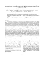
42] The results of performing this analysis for Y =
acetone, MEK and acetaldehyde are shown in Figure 5.
Each solid line shows the coefficient of determination
between an individual combustion marker and c
yo
,asa
function of the value of (Y/TOL)
E
that was used to calculate
c
yo
. The c ompounds used as markers of combustion
(V, with mixing ratios c
v
) were those VOCs thought to
Figure 5. Coefficient of determination between combus-
tion or photochemically derived VOCs and the residual term
c
yo
, representing photoch emical and biogenic OVOC
sources, as a fu nction of the primary emission ratio
(Y/TOL)
E
. Each solid (dashed) line represents a separate
combustion (photochemical) marker compound (V, with
mixing ratio c
v
, for V = propyne, 2-methylpropene,
t-2-butene, c-2-bu tene, 2- methyl-1-but ene, 3 -methyl-1-
butene, t-2-pentene, benzene, ethylbenzene, p-xyle ne,
m-xylene, o-xylene, NO
x
, MACR, or MVK). The critical
point in the curves gives the combustion emission ratio for
species Y (acetone, MEK, or acetaldehyde) relative to toluene.
D07S07 MILLET ET AL.: VOLATILE ORGANICS AT THE PITTSBURGH SUPERSITE
9of17
D07S07
be solely or predominantly derived via combustion pro-
cesses (propyne, 2-methylpropene, t-2-butene, c-2-butene,
2-methyl-1-butene, 3-methyl-1-butene, t-2-pentene,
benzene, ethylbenzene, p-xylene, m-xylene, o-xylene) and
NO
x
. Dashed lines show r
2
between c
yo
and VOCs thought
to be solely photochemically produced (MACR and MVK,
which were present above detection limit in the summer
experiment only), as a function of (Y/TOL)
E
.
[
43] There is a well defined minimum in the curve for the
combustion markers, the location of which, for a given
oxygenated VOC species Y, is consistent across all marker
compounds. For the summer data, the location of this
minimum coincides with the maximum r
2
value for the
photochemically produced tracer species. We interpret the
location of the critical value of r
2
as the representative (Y/
TOL)
E
value for that time of year (Table 4).
[
44] Primary emission ratios, relative to toluene, for
acetone, MEK and acetaldehyde were all substantially
(1.4–2.4 times) higher in January – February 2002 than in
July–August 2002. Since the emission ratio depends on the
toluene as well as OVOC emission strength, seasonal
changes in the emission ratio can be due to changes in the
numerator, denominator or both. This issue is discussed
further in the following section. The primary emission ratios
calculated in this section are averages over the sources
impacting the air masses that were sampled during the
course of the study. They therefore represent integrated
regional emission ratios for Pittsburgh in January – February
and July–August 2002.
[
45] Urban and industrial VOC emission ratios depend on
a number of factors, in particular vehicle fleet and fuel
characteristics as well as types of industrial activity in the
region. Such variability complicates efforts to construct
reliable emission inventories for use in air quality modeling,
and emphasizes the utility of the approach developed here,
which provide s top-down observational c onstraints on
regional pollutant emission ratios. On-road studies of motor
vehicle exhaust in the U.S. (generally carried out during
summer) report emission ratios for acetone, MEK and
acetaldehyde relative to toluene ranging from 2 –4%, 2–
12%, and <1–8% (molar basis) respectively for light-duty
vehicles [Kirchstetter et al., 1999; Fraser et al., 1998;
Zielinska et al., 1996; Kirchstetter et al., 1996]. Heavy-duty
or diesel vehicles emit substantially higher amounts of these
OVOCs relative to toluene, with emission ratios frequently
greater than unity [Zielinska et al., 1996; Staehelin et al.,
1998]. Inventory estimates (including mobile, point and
nonpoint sources) of annual acetaldehyde and MEK emis-
sions in Allegheny County are 14% and 10% those of
toluene respectively on a molar basis (see .
gov/ttn/chief/net/index.html), substantially lower than the
values determined here (Table 4). If inventory estimates of
toluene emissions are accurate, this suggests that acetalde-
hyde and MEK emissions are underestimated by factors of
approximately 3.8 and 2.6 (from the average of the summer
and winter ratios, Table 4).
[
46] For the summer data, c
yo
for both acetone and MEK
exhibited a well-defined maximum correlation with MACR
and MVK (Figure 5), indicating that the other, noncombus-
tive, source represented by c
yo
is likely to be largely
photochemical. For acetaldehyde, the poor correlation of
c
yo
with MACR and MVK suggests that c
yo
is not
exclusively photochemical in nature, and may contain
another significant component such as biogenic emissions.
[
47] For comparison, Figure 6 shows results of the same
analysis for Y = MACR and MVK, species whose only
significant known source is from photochemical oxidation
of isoprene. In this case, the minimum correlation of c
yo
with combustion derived VOCs (and maximum correlation
with MVK or MACR) occurs at a combustion emission
ratio (Y/TOL)
E
of zero, showing that there are no significant
primary emissions of these compounds.
[
48] With (Y/TOL)
E
determined by the critical points in
Figure 5, the contributions to the concentration of species Y
from background (c
a
), combustion emissions (c
yc
), and
other sources (c
yo
) as a function of time can then be
calculated from (2) and (3). Contributions of c
a
, c
yc
, and
c
yo
to the ambient levels of acetone, MEK, and acetalde-
hyde in summer and winter are summarized in Table 4.
Negative values of c
yo
were assumed to contain no sec-
ondary or biogenic material and were set to zero.
[
49] Ambient concentrations of acetone, MEK and acet-
aldehyde during summer were on average 3–4 times higher
than winter (Table 4). Increases in background concentra-
tions were responsible for a significant portion of this winter
to summer difference, with summer background levels on
average 2.5–5 times higher than in the winter. However, the
fraction of the total concentration due to the background
was comparable in summer and winter. In both seasons, the
background made up, on average, slightly over half of the
Table 4. OVOC Combustion Emission Ratios and Source Contributions
a
Species (Y)
Ambient
Concentration
Primary Emission
Ratio
Background
Concentration Combustion Emissions Other Sources
c
y
, ppt
(Y/TOL)
E
c
a
,
ppt
c
a
/c
y
c
yc
, ppt c
yc
/c
y
c
yo
, ppt c
yo
/c
y
Median IQR
b
Median IQR
b
Median IQR
b
Median IQR
b
Median IQR
b
Median IQR
b
Median IQR
b
Winter
Acetone 943 655 – 1390 0.78 0.74 – 0.82 526 0.56 0.38 – 0.80 114 49 – 241 0.12 0.05 – 0.21 237 23 – 624 0.24 0.04 – 0.48
MEK 215 153 –299 0.34 0.34 – 0.34 120 0.56 0.40 – 0.79 50 21 – 105 0.23 0.10 – 0.39 24 0 –92 0.12 0.00 – 0.35
Acetaldehyde 538 403–729 0.62 0.60 – 0.64 289 0.54 0.40 – 0.72 91 39 – 192 0.17 0.07 – 0.31 146 24 – 290 0.27 0.05 – 0.40
Summer
Acetone 4030 3130 – 4890 0.32 0.29 – 0.34 2650 0.66 0.54 – 0.85 81 29 – 224 0.02 0.01 – 0.06 1200 353 – 1940 0.29 0.12 – 0.41
MEK 559 408 –674 0.17 0.16 – 0.18 319 0.57 0.47 – 0.78 45 16 – 123 0.10 0.03 – 0.23 138 29 – 257 0.26 0.06 – 0.40
Acetaldehyde 1560 1100–2150 0.43 0.40–0.52 798 0.51 0.37 –0.72 113 40–310 0.09 0.03 –0.20 542 126 – 1050 0.34 0.11–0.50
a
Note that the median values of the source contributions do not necessarily add up to the median ambient concentration as the median is not a distributive
property.
b
IQR, interquartile range.
D07S07 MILLET ET AL.: VOLATILE ORGANICS AT THE PITTSBURGH SUPERSITE
10 of 17
D07S07
overall abundance for all three compounds (Table 4). The
higher summer background concentrations for these species
were probably due to increased nonlocal photochemical
production and biogenic emission during that time of year.
[
50] The absolute contribution from combustion to atmo-
spheric mixing ratios was very similar in summer and
winter, despite the large changes in emission ratios (which
were higher in winter by factors of 2.4, 2.0 and 1.4 for
acetone, MEK and acetaldehyde; see discussion in follow-
ing section). However, total concentrations were substan-
tially higher in summer, and combustion emissions were a
significantly smaller fraction of the total source (Table 4).
[
51] Other sources, which we assume to be predominantly
photochemical but which also likely include some biogenic
emissions in summer, were substantially higher in summer
for all three compounds. Median summer values of c
yo
were over 5 times higher than in winter for acetone and
MEK and nearly 4 times higher for acetaldehyde.
[
52] With the exception of MEK, combustion was not the
major source of these compounds, even in winter. For MEK,
combustion emissions were more important than other
sources (c
yo
) in the winter (a median of 23% versus
13%). This was not the case in the summer, however, nor
was it true for acetone or acetaldehyde in either season. For
acetone, other sources were twice as important as combus-
tion emissions in the winter and ten times as important in
the summer. For acetaldehyde, other sources were 50%
larger than combustion emissions in winter and 4 times
larger in summer.
[
53] Diurnally averaged OVOC source contributions,
overlaid with ozone concentrations, in winter and summer
are shown in Figure 7. For the summer data set, the other
OVOC sources (c
yo
) showed a strong photochemical sig-
nature: low at night, increasing after sunrise and peaking in
the afternoon. For each compound, acetone, MEK and
acetaldehyde, the c
yo
term tracked ozone quite closely.
For the winter data set, the c
yo
terms for each OVOC
showed a much weaker photochemical signal, and the
relative contribution from combustion was substantially
larger than in the summer. Note that since c
yc
for each
Figure 6. Same as Figure 5, except for Y = methacrolein
(MACR) and methylvinylketone (MVK). The minimum
correlation of c
yo
with combustion derived VOCs (and
maximum correlation with photochemical VOCs) occurs at
an emission ratio (Y/TOL)
E
of zero, showing that there are
no significant primary emissions of these compounds.
Figure 7. Diurnal patterns in OVOC source contributions (winter and summer data). Combustion
source (c
yc
, ppb), pluses and unshaded region; photochemical and biogenic sources (c
yo
, ppb), circles
and surrounding gray area. Ozone is also shown (solid dark line). Points show median values; banded
areas show the interquartile range. Note different y axis scales for winter and summer.
D07S07 MILLET ET AL.: VOLATILE ORGANICS AT THE PITTSBURGH SUPERSITE
11 of 17
D07S07
OVOC is defined as c
tol
(Y/TOL)
E
, i.e. the observed toluene
enhancements multiplied by a primary emission ratio,
diurnal patterns in c
yc
shown in Figure 7 reflect that of
toluene.
3.3.2. Choice of Combustion Marker and Seasonal
Patterns in Emission Ratios
[
54] Repeating the above analysis using other combustion
derived compoun ds instead of toluene as the pr imary
emission tracer resulted in only minor changes to the
calculated OVOC partitioning (Table 4) and did not alter
any of the conclusions. This gives us confidence that this
approach to partitioning VOC source contributions is
robust. For a given primary emission tracer, the calculated
OVOC emission ratios, given by the critical r
2
,were
consisten t using compounds that are solely combustion
derived (e.g. alkenes and alkynes) and compounds that
have additional anthropogenic noncombustion sources, such
as evaporative losses and chemical processing (e.g. benzene
and toluene). Hence the approach is not sensitive to slight
differences in source profiles for the marker compounds. We
conclude that the calculated emission ratios represent an
integrated regional primary pollution signal, rather than one
specific source type.
[
55] In addition, we note that the combustion markers
employed to calculate the OVOC primary emission ratios
relative to toluene (Figure 5) have lifetimes that vary by
nearly a factor of 50, yet they give consistent emission ratio
estimates. This may indicate that much of the variability
observed is relatively local and not driven by photochemical
lifetime or by the different sampling footprints for species of
different lifetimes.
[
56] Seasonal differences in the OVOC primary emission
ratios, however, calculated relative to the tracer compound,
changed dramatically depending on the tracer used. This is
to be expected since t he primary emission ratios are
sensitive to changes in both the numerator and denominator,
and different combustion tracers do not necessarily have
identical seasonal patterns in emission strength. While the
primary OVOC emission ratios relative to toluene were all
higher in the winter, OVOC emission ratios calculated
relative to alkenes and alkynes were generally 2–3 times
higher in the summer. It is possible that noncombustion
toluene sources, i.e. evaporative emissions, are higher in
summer which would decrease the OVOC emission ratio for
that time of year. However, the short-lived alkenes are
oxidized much more rapidly in the summer months due to
higher concentrations of OH and ozone. Over a given
source-receptor distance, then, the alkenes would be more
depleted relative to the OVOCs in the summer than in the
winter. This would lead to higher OVOC:alkene emission
ratios in the summer, as observed. While this effect would
also occur with toluene, either the effect was small due to
toluene’s longer lifetime (10 times that of t-2-butene) and/or
it was offset by increased emissions.
3.3.3. Quantification of Secondary Organic Aerosol
[
57] Organic carbon (OC) constitutes a significant frac-
tion of atmospheric aerosol [Lim and Turpin, 2002; Cabada
et al., 2002, 2004; Tolocka et al., 2001]; however, its origin
and composition remain poorly understood. OC consists of
hundreds or thousands of individual organic compounds.
Both anthropogenic sources (e.g. combustion) and biogenic
sources (e.g. plants) can contribute to aerosol organic
carbon via direct emission of particles (primary OC), and
via emission of gas-phase precursor compounds that parti-
tion into the aerosol phase upon oxidation (secondary OC).
Clarifying the roles of primary and secondary OC produc-
tion is an important step toward an improved understanding
and modeling of the sources, morphology and effects of
aerosol OC. The technique of minimizing (maximizing) the
correlation between combustion (photochemical) tracer
compounds and the photochemical component of a species
of interest, developed in the previous section, also has utility
in determining the primary emission ratio for pollutants
other than VOCs. Here, we apply the method to quantify the
relative importance of primary and secondary OC sources in
the study region.
[
58] As above, aerosol organic carbon concentrations
(M
oc
,inmg of carbon per cubic meter, mgC/m
3
) are defined
as being composed of combustion (M
c
) and other (M
o
)
components, plus a regional background (M
a
)[Turpin and
Huntzicker, 1995]:
M
oc
¼ M
c
þ M
o
þ M
a
: ð4Þ
[59] Elemental carbon (EC, or soot) is an aerosol com-
ponent whose only source is direct emission from combus-
tion. If both OC and EC are emitted from primary sources
according to a characteristic averaged OC:EC emission ratio
(OC/EC)
E
, then the combustion-derived organic carbon can
be estimated as
M
c
¼ M
ec
OC
EC
E
; ð5Þ
where M
ec
represents elemental carbon enhancements above
background (in mgC/m
3
), and M
o
is given by
M
o
¼ M
oc
À M
ec
OC
EC
E
À M
a
: ð6Þ
[60] The background term, M
a
, represents noncombustion
primary OC (e.g. from biogenic sources) as well as any
regional aerosol organic carbon background. As above, we
estimate M
a
as the 0.1 quantile of the measured OC
concentrations. M
o
is then assumed to be exclusively
secondary OC. It should be pointed out, however, that if
there exist significant sources of primary OC which do not
correlate with EC and are highly variable through time (and
thus are not entirely captured by the M
a
parameter), then M
o
may also contain some primary influence.
[
61] One challenge associated with the EC tracer method
as it has been applied in the past involves defining the
OC:EC ratio of primary emissions, as this can vary signif-
icantly between sources and consequently as a function of
time. In addition, defining (OC/EC)
E
from ambient OC and
EC concentration data requires that there be a subset of data
with no significant secondary contributions to the measured
OC concentrations. The typical approach is to qualitatively
eliminate data points that are likely to be impacted by
significant secondary production or other factors such as
rain events, and regress OC on EC for that subset of data
dominated by primary OC [Turpin and Huntzicker, 1995;
Cabada et al., 2004]. This then gives a regression slope that
is in theory reflective solely of primary emissions. The
D07S07 MILLET ET AL.: VOLATILE ORGANICS AT THE PITTSBURGH SUPERSITE
12 of 17
D07S07
parameter M
a
, reflecting primary noncombustion OC, is then
assumed to be constant and given by the intercept, enabling
the calculation of M
o
. In the event of significant temporal
variability inthe primary OC:EC ratioimpacting the sampling
site, this process may be repeated on subsets of the data.
[
62] Here we employ the tec hnique developed in the
previous section, using the range of markers for primary
and secondary processes provided by the VOC data set to
define the characteristic OC:EC primary emission ratio for the
Pittsburgh region in summer and winter. This approach
avoids the need to carefully select time periods that will yield
the ‘‘correct’’ value of (OC /EC)
E
. In addition, the suite of
primary and secondary VOCs available provides bounds on
the value of (OC/EC)
E
appropriate to a given time period. The
secondary organic aerosol is then calculated according to (6).
[
63] The coefficient of determination between M
o
and
combustion and photochemically derived VOCs is shown in
Figure 8 as a function of (OC/EC)
E
for winter and summer.
Again, the critical point of the curves gives the representa-
tive value of (OC/EC)
E
for that time of year.
[
64] The median value of (OC/EC)
E
determined for the
winter data set was 1.85 (IQR: 1.82–1.86), whereas that for
the summer data set was lower with a median of 1.36 (IQR:
1.27–1.48) (Table 5). Substantially higher particulate con-
centrations of levoglucosan were observed in the winter,
indicative of increased wood combustion. More widespread
wood burning is a likely cause of the higher primary OC:EC
emission ratio at that time of year. Colder engine s and less
efficient combustion may have also contributed to the
higher wintertime ratio.
[
65] Using the derived values of (OC/EC)
E
for summer
and winter, we can then calculate M
o
, the secondary OC,
according to (6). Timelines of the total (M
oc
), combustion
(M
c
), and secondary (M
o
) aerosol organic carbon concen-
trations (in mgC/m
3
) for winter and summer 2002 are plotted
in Figure 9, and quantiles of these quantities are given in
Table 5. Note that since M
c
is defined as M
ec
(OC/EC)
E
,
there are occasional episodes where M
c
> M
oc
. Negative
values of M
o
were assumed to contain no secondary
material and were set to zero.
[
66] Ambient concentrations of aerosol organic carbon in
the summer experiment were on average twice as high as in
the winter (Table 5). Background levels (M
a
) made up a
significant fraction of the total ambient aerosol OC concen-
trations in both seasons. Background aerosol OC concen-
trations were slightly higher in summer but a larger fraction
of the total in winter (median of 49% versus 35%).
Similarly, combustion OC was slightly higher in the sum-
mer, however, it made up a larger fraction of the total OC in
winter (median of 30% versus 19%). Secondary organic
carbon ( M
o
) accounted for a median of 16% (IQR: 0 –35%)
of the aerosol OC in winter, and 37% (IQR: 15 – 56%) in
summer (Table 5).
[
67] A. Polidori et al. (manuscript in preparation, 2005)
carried out an analysis of the primary and secondary
components of OC in Pittsburgh during the PAQS study
Figure 8. Coefficient of determination between combus-
tion or photochemically derived VOCs and the residual term
M
o
, representing secondary OC, as a function of the primary
emission ratio (OC/EC)
E
. Each solid (dashed) line repre-
sents a separate combustion (photochemical) marker
compound. The critical point in the curves gives the
primary emission ratio (OC/EC)
E
.
Table 5. OC Combustion Emission Ratios and Source Contributions
a
Season
Ambient
Concentration
Primary
Emission
Ratio
Background
Concentration Combustion Emissions Secondary Production
M
oc
,
mgC/m
3
(OC/EC)
E
M
a
,
mgC/m
3
M
a
/M
oc
M
c
,
mgC/m
3
M
c
/M
oc
M
o
,
mgC/m
3
M
o
/M
oc
Median IQR
b
Median IQR
b
Median IQR
b
Median IQR
b
Median IQR
b
Median IQR
b
Median IQR
b
Winter 1.2 0.83–2.0 1.85 1.82 – 1.86 0.60 0.49 0.30– 0.72 0.37 0.13 – 0.75 0.30 0.13–0.48 0.20 0.00 – 0.59 0.16 0.00–0.35
Summer 2.5 1.6 – 3.9 1.36 1.27–1.48 0.87 0.35 0.22–0.54 0.50 0.20–1.1 0.19 0.10 – 0.32 0.99 0.27–1.9 0.37 0.15 – 0.56
a
Note that the median values of the source contributions do not necessarily add up to the median ambient concentration as the median is not a distributive
property.
b
IQR, interquartile range.
Figure 9. Timelines of total OC (M
oc
, mgC/m
3
), dark solid
line; combustion OC (M
c
, mgC/m
3
), dashed line; secondary
OC (M
o
, mgC/m
3
), light solid line. Data are shown for the
(a) winter and (b) summer deployments.
D07S07 MILLET ET AL.: VOLATILE ORGANICS AT THE PITTSBURGH SUPERSITE
13 of 17
D07S07
using the Turpin and Huntzicker [1995] EC tracer method.
For overlapping time periods (10 January to 12 February
and 10 –31 July 2002), they calculate median secondary
OC concentrations of 0.21 mgC/m
3
(15% of total OC) and
1.04 mgC/m
3
(47% of total OC) respectively. These
values are in good agreement with those calculated here
for the same periods: 0.20 mgC/m
3
(16% of total OC) and
1.15 mgC/m
3
(43% of total OC) (note that these values differ
slightly from those in Table 5 since they do not reflect
identical time periods).
3.4. Characterization of the Chemical State of the
Atmosphere: VOC Contributions to OH Loss
[
68] Photochemical production of secondary organic
aerosol (SOA) depends on the chemical state of the atmo-
sphere, both in terms of oxidative capacity, and in term of
the quantity and nature of gas phase organic material that is
present to form aerosol. In this section we describe the
relative importance of different classes of VOCs to tropo-
spheric photochemistry in the Pittsburgh region in summer
and winter, and show that higher levels of photochemically
active compounds are present in summer, when SOA levels
are highest, due to biogenic emissions and photochemical
production of OVOCs.
[
69] A useful measure of air mass chemical reactivity is
the OH loss rate (L
OH
,s
À1
), defined as
L
OH
¼
X
i
k
i
c
i
; ð7Þ
where k
i
is the reaction rate constant for species i with the
hydroxyl radical [Atkinson, 1994], and c
i
is the concentra-
tion of i in molec/cm
3
.L
OH
has units of s
À1
and represents
the inverse lifetime of the hydroxyl radical with respect to
reaction with the measured compounds.
[
70] Daytime (1000–1600 EST) values of L
OH
were
calculated for the following groups of compounds: total
(all measured VOCs plus CO); alkanes; alkenes + alkynes;
aromatics; OVOCs; isoprene plus its oxidation products
methacrolein, methylvinylketone, and 3-methylfuran; and
CO (Figure 10; Tables 6 and 7).
[
71] Due to analytical challenges, VOC measurements in
many field studies of air quality and atmospheric chemistry
comprise only the anthropogenic nonmethane hydrocarbons
(NMHCs; alkanes, alkenes, alkynes and aromatics). In
Pittsburgh during January and February 2002, these species
accounted for a substantial portion (approximately 60%) of
the total measured OH loss rate. However, while t heir
collective OH reactivity was only slightly less in summer
(0.68 s
À1
versus 0.89 s
À1
), their importance relative to other
VOCs was dramatically lower, as they accounted for only
11% on average of total L
OH
during summer. Similarly, the
CO reactivity was comparable in both seasons (median of
0.49 s
À1
in winter and 0.53 s
À1
in summer), but its relative
contribution to the total measured OH loss rate was much
greater in winter (median of 23% versus 7% in the summer).
It should be pointed out that these calc ulations do not
include the C
2
hydrocarbons ethane, ethene and ethyne ,
which were not measured. Based on published ratios of
these compounds to other species [Parrish et al., 1998], we
estimate that they would cause an OH loss rate of approx-
imately 0.05 s
À1
and 0.13 s
À1
for summer and winter.
[
72] Despite the comparable NMHC and CO reactivity in
the two seasons, the total measured daytime OH loss rate
underwent a more th an fourfold incr ease from win ter
(median = 1.42 s
À1
;IQR:1.12–2.30s
À1
)tosummer
(median = 7.25 s
À1
; IQR: 4.60–9.38 s
À1
). This was due
to the presence of high levels of isoprene and its oxidation
products in summer, and also to the three-fold increase in
oxygenated VOC concentration and reactivity from winter
to summer (Tables 6, 7). Isoprene plus its oxidation prod-
ucts accounted for a median of 62% (IQR: 52–70%) of the
daytime OH loss rate in summer, with the OVOCs account-
ing for an additional 20% (IQR: 15–26%). Formaldehyde
measurements were not made during the PAQS study, and
including the effects of this compound would result in an
increased contribution to the calculated OH loss rate from
the OVOCs in both seasons.
[
73] The PAQS sampling site was located at the north end
of Schenley Park, a 456 acre urban park with substantial
tree cover. To test whether the observed isoprene concen-
trations were biased by the presence of a large nea rby
source, the daytime OH loss due to isoprene and its
Figure 10. Probability density curves of measured day-
time (1000 –1600 EST) VOC OH loss rate by compound
class for winter and summer 2002. Measured OH loss rate
for isoprene plus its oxidation products methacrolein,
methylvinylketone, and 3-methylfuran is shown for both
hot (maximum air temperature ! 29°C) and cool (maximum
air temperature < 29°C) days in the summer. These
compounds were not present above detection limit in the
winter. Note the different scales for the x axes in the left-
and right-hand columns.
D07S07 MILLET ET AL.: VOLATILE ORGANICS AT THE PITTSBURGH SUPERSITE
14 of 17
D07S07
oxidation products was calculated for time periods when the
wind was only from the northern sector and the wind speed
was greater than 1 m/s. The resulting OH loss rate (median
4.55 s
À1
; IQR 2.85 – 5.73 s
À1
) was not significantly differ-
ent from that calculated using all of the daytime data
(median 4.71 s
À1
; IQR 2.77–6.20 s
À1
). Hence we find that
in winter, the total daytime OH loss rate is dominated by the
nonmethane hydrocarbons and CO, whereas in summer it is
dominated by isoprene, its oxidation products, and oxygen-
ated VOCs. The above calculations do not include methane,
Table 6. Quantiles of Daytime OH Loss Rate: Winter Data
a,b
Category
All Days High Ozone Days
c
L
OH
,s
À1
Fraction of Total VOC
L
OH
L
OH
,s
À1
Fraction of Total VOC
L
OH
Median IQR
e
Median IQR
e
Median IQR
e
Median IQR
e
Total 1.42 1.12 –2.30 1.00 0.91 – 1.27
Alkanes
f
0.31 0.25–0.41 0.20 0.17 – 0.25 0.27 0.17 – 0.32 0.20 0.18 – 0.26
Alkenes + Alkynes
f
0.41 0.32–0.57 0.27 0.23 – 0.32 0.29 0.23 – 0.40 0.25 0.22 – 0.30
Aromatics 0.17 0.12–0.23 0.11 0.09– 0.13 0.12 0.09 – 0.19 0.10 0.09 – 0.12
OVOCs 0.41 0.33–0.57 0.29 0.23–0.35 0.45 0.31–0.54 0.38 0.29 – 0.45
CO 0.49 0.21 –1.05 0.23 0.17–0.36 0.19 0.19 – 0.19 0.20 0.20 – 0.22
Category
High OC Days
c
Nucleation Days
d
L
OH
,s
À1
Fraction of Total VOC
L
OH
L
OH
,s
À1
Fraction of Total VOC
L
OH
Median IQR
e
Median IQR
e
Median IQR
e
Median IQR
e
Total 2.70 1.64 –3.35 1.04 0.98 – 1.20
Alkanes
f
0.40 0.33–0.58 0.18 0.14 – 0.20 0.26 0.24 – 0.30 0.27 0.21 – 0.29
Alkenes + alkynes
f
0.57 0.44–0.84 0.24 0.20 – 0.30 0.28 0.26 – 0.35 0.28 0.25 – 0.31
Aromatics 0.25 0.14–0.31 0.09 0.07– 0.11 0.12 0.10 – 0.16 0.11 0.09 –0.13
OVOCs 0.69 0.51–0.78 0.26 0.21–0.32 0.37 0.34–0.45 0.35 0.32 – 0.38
CO 0.74 0.45 –1.56 0.28 0.16–0.36 <DL
g
<DL
g
<DL
g
<DL
g
a
Note that the median values of the components do not necessarily add up to the median of the total as the median is not a distributive property.
b
Daytime: 1000 –1600 EST.
c
High ozone and high OC days are defined as days when the daily maximum concentration was above the 0.8 quantile for all daily maxima.
d
Days on which moderate to strong nucleation events occurred [Stanier et al., 2004b].
e
IQR, interquartile range.
f
Note that ethane, ethene, and ethyne were not measured. See text for discussion.
g
CO concentrations during these periods were below the instrumental detection limit of 0.1 ppm.
Table 7. Quantiles of Daytime OH Loss Rate: Summer Data
a,b
Category
All Days High Ozone Days
c
L
OH
,s
À1
Fraction of Total VOC
L
OH
L
OH
,s
À1
Fraction of Total VOC
L
OH
Median IQR
e
Median IQR
e
Median IQR
e
Median IQR
e
Total 7.25 4.60–9.38 8.53 7.17– 9.77
Alkanes
f
0.17 0.12–0.24 0.03 0.02–0.04 0.19 0.17 – 0.30 0.03 0.02 –0.04
Alkenes + alkynes
f
0.36 0.30–0.45 0.06 0.04 – 0.07 0.42 0.36–0.51 0.05 0.04 – 0.06
Aromatics 0.14 0.08–0.24 0.02 0.01 – 0.04 0.13 0.08 – 0.24 0.02 0.01–0.03
OVOCs 1.35 1.09– 1.64 0.20 0.15 –0.26 1.80 1.53–1.97 0.21 0.16 – 0.24
Isop + Ox
f
4.71 2.77–6.20 0.62 0.52 – 0.70 5.69 3.75–6.67 0.63 0.58 – 0.71
CO 0.53 0.26–0.86 0.07 0.04–0.12 0.60 0.24 – 0.83 0.06 0.03 – 0.09
Category
High OC Days
c
Nucleation Days
d
L
OH
,s
À1
Fraction of Total VOC
L
OH
L
OH
,s
À1
Fraction of Total VOC
L
OH
Median IQR
e
Median IQR
e
Median IQR
e
Median IQR
e
Total 9.26 8.23 – 10.43 4.96 3.37 – 6.47
Alkanes
f
0.21 0.16–0.27 0.03 0.02 – 0.04 0.11 0.09 – 0.20 0.03 0.02 –0.03
Alkenes + alkynes
f
0.38 0.31–0.48 0.04 0.04 – 0.06 0.35 0.25–0.43 0.07 0.06 – 0.07
Aromatics 0.27 0.19–0.40 0.03 0.02 – 0.05 0.12 0.08 – 0.14 0.02 0.02–0.03
OVOCs 1.54 1.35– 1.84 0.17 0.14 –0.20 1.30 1.05–1.59 0.26 0.23 – 0.30
Isop + Ox
g
5.71 4.58–6.75 0.64 0.57 – 0.70 3.16 1.91–3.92 0.59 0.52 – 0.62
CO 0.71 0.57–1.04 0.09 0.07 – 0.11 0.22 0.16–0.54 0.07 0.02 – 0.09
a
Note that the median values of the components do not necessarily add up to the median of the total as the median is not a distributive property.
b
Daytime: 1000 –1600 EST.
c
High ozone and high OC days are defined as days when the daily maximum concentration was above the 0.8 quantile for all daily maxima.
d
Days on which moderate to strong nucleation events occurred [Stanier et al., 2004b].
e
IQR, interquartile range.
f
Note that ethane, ethene, and ethyne were not measured. See text for discussion.
g
Isoprene plus its oxidation products MACR, MVK, and 3-methylfuran.
D07S07 MILLET ET AL.: VOLATILE ORGANICS AT THE PITTSBURGH SUPERSITE
15 of 17
D07S07
which was not measured during the experiment. Based on
background concentrations of methane at this latitude (see
http://ww w.cmdl.noaa.gov/info/ftpdata.html) , we estimate
the OH loss rate in Pittsburgh due to methane at approxi-
mately 0.21 s
À1
during the winter and 0.32 s
À1
during the
summer.
[
74] Daytime OH loss rates were also calculated on the
following subsets of t he data: high ozone days, high aerosol
OC days, and days in which moderate to strong nucleation
events were observed [Stanier et al., 2004b] (Tables 6
and 7). High ozone and high OC days were defined as days
in which the maximum value of these quantities was above
the 0.8 quantile for all observed daily maxima.
[
75] For July and August, the 0.8 concentration quantile
for the daily maximum ozone was 84 ppb. On high ozone
days, the total measured OH loss rate was higher (median:
8.53 s
À1
) than otherwise (days not exceeding this threshold
had a median OH loss rate of 6.74 s
À1
), and this increase
was distributed relatively evenly among the different com-
pound classes (Table 7). During January and February, the
0.8 quantile for daily ozone maxima was only 30 ppb. Days
during which ozone exceeded this amount had a lower
overall OH loss rate (median 1.00 s
À1
) than days on which
it did not (median 1.57 s
À1
). These higher ozone days in the
winter may have occurred during periods of enhanced
vertical mixing. Comrie and Yarnal [1992] analyzed the
dependence of surface ozone in Pittsburgh on synoptic
climatology. They concluded that high ozone leve ls in
summer developed under stagnant anticyclonic cond itions,
whereas in winter high ozone concentrations were associ-
ated with tropopause folding and vertical transport of
stratospheric ozone.
[
76] In both seasons, days with high OC loadings were
associated with higher levels of all VOC compound cate-
gories and CO. In January – February, the median OH loss
rate was 2.70 s
À1
on days with high OC versus 1.28 s
À1
on
days without. In July–August, the median daytime OH loss
rate was 9.26 s
À1
on high OC days and 6.81 s
À1
on other
days. By contrast, days on which nucleation events occurred
had lower overall OH loss rates (medians of 1.04 s
À1
and
4.96 s
À1
in winter and summer, respectively) than days
without nucleation events (medians of 1.54 s
À1
and 7.93 s
À1
in winter and summer). Stanier et al. [2004b] found that the
occurrence of nucleation events during PAQS was depen-
dent on the preexisting aerosol surface area available for
condensation. The lower OH loss rates on nucleation days
may be due to a positive correlation between gas phase
reactivity and aerosol surface area (r
2
= 0.48 in winter and
0.28 in summer); i.e. less polluted days with low OH loss
rates also had lower particle surface area available for
condensation of semivolatile aerosol precursors, which
increased the likelihood of new particle nucleation.
4. Conclusions
[77] High temporal density speciated VOC measurements
provide a useful framework for interpreting aerosol mea-
surements. Statistical analyses such as factor analysis on
combined VOC-aerosol data sets can test precepts used in
source-receptor modeling. The range of combustion and
photochemical markers in the VOC data set also enables us
to deconvolve the relative contributions to ambient levels of
OVOCs and aerosol OC from different source types. We
calculate that secondary plus biogenic sources accounted for
24%, 12% and 27% of the ambient concentrations of
acetone, MEK and acetaldehyde respectively in the winter
and 29%, 26% and 34% respectively in the s ummer.
Aerosol OC was found to be composed of 16% secondary
carbon in the winter and 37% secondary carbon in the
summer. The importance of the background contribution to
observed concentrations of both OVOCs and aerosol OC
emphasizes the role of longer-range transport and the need
for a regional perspective i n addressing air quality concerns.
While local automotive emissions were the primary factor
driving changes in VOC concentrations in Pittsburgh,
they did not contribute significantly to variability in the
aerosol species included in the factor analysis (PM 2.5
mass, aerosol sulfate and nitrate mass, and aerosol number
density).
[
78] VOC concentration data can also help define chem-
ical conditions that are conducive to particle formation and
growth. We find that while aerosol OC loadings are highest
when VOC concentrations and reactivities are high, nucle-
ation events tended to occur on days when levels of VOCs
and CO were low. High ozone days in the summer were
associated with high OH loss rates due to the VOCs and
CO, whereas in the winter the highest ozone levels occurred
on days with low levels of CO and nonmethane hydro-
carbons but slightly higher OVOC concentrations.
[
79] One of the overall objectives of the PAQS study is to
develop the ability to predict changes in PM characteristics
and atmospheric composition due to proposed changes in
emissions. Reaching this objective will require accurate
modeling of the chemical and dynamical processes control-
ling atmospheric composition in the Pittsburgh region. The
results presented here should help to provide a basis upon
which to test mechanisms included in such models.
[
80] Acknowledgments. This research was conducted as part of the
Pittsburgh Air Quality Study, which was supported by the US EPA under
contract R82806101 and the US DOE National Energy Technology
Laboratory under contract DE-FC26-01NT41017. DBM thanks the DOE
for a GREF fellowship. The authors thank all of the PAQS researchers for
their help; in particular, Allen Robinson, Beth Wittig, and Andrey Khlystov.
Thanks also to Megan McKay for her considerable help.
References
Atkinson, R. (1994), Gas phase tropospheric chemistry of organic com-
pounds, J. Phys. Chem. Ref. Data Monogr., 2, 1–216.
Bakwin, P. S., D. F. Hurst, P. P. Tans, and J. W. Elkins (1997), Anthropo-
genic sources of halocarbons, sulfur hexafluoride, carbon monoxide, and
methane in the southeastern United States, J. Geophys. Res., 102(D13),
15,915 –15,925.
Barnes, D. H., S. C. Wofsy, B. P. Fehlau, E. W. Gottlieb, J. W. Elkins, G. S.
Dutton, and S. A. Montzka (2003), Urban/industrial pollution for the
New York City – Washington, D. C., corridor, 1996 – 1998: 1. Providing
independent verification of CO and PCE emissions inventories, J. Geo-
phys. Res., 108(D6), 4185, doi:10.1029/2001JD001116.
Cabada, J. C., S. N. Pandis, and A. L. Robinson (2002), Sources of atmo-
spheric carbonaceous particulate matter in Pittsburgh, Pennsylvania, J. Air
Waste Manage., 52(6), 732 – 741.
Cabada, J. C., S. Takahama, A. Khlystov, S. N. Pandis, S. Rees, C. I.
Davidson, and A. L. Robinson (2004), Mass size distributions and size
resolved chemical composition of fine particulate matter at the Pittsburgh
Supersite, Atmos. Environ., 38(20), 3127 – 3141.
Comrie, A. C., and B. Yarnal (1992), Relationships between synoptic-
scale atmospheric circulation and ozone concentrations in metropolitan
Pittsburgh, Pennsylvania, Atmos. Environ., 26(3), 301–312.
Czoschke, N. M., M. Jang, and R. M. Kamens (2003), Effect of acidic seed
on biogenic secondary organic aerosol growth, Atmos. Environ., 37(30),
4287 – 4299.
D07S07 MILLET ET AL.: VOLATILE ORGANICS AT THE PITTSBURGH SUPERSITE
16 of 17
D07S07
Fraser, M. P., G. R. Cass, and B. R. T. Simoneit (1998), Gas-phase and
particle-phase organic compounds emitted from motor vehicle traffic
in a Los Angeles roadway tunnel, Environ. Sci. Technol., 32(14),
2051 –2060.
Goldan, P. D., M. Trainer, W. C. Kuster, D. D. Parrish, J. Carpenter, J. M.
Roberts, J. E. Yee, and F. C. Fehsenfeld (1995a), Measurements of
hydrocarbons, oxygenated hydrocarbons, carbon monoxide, and nitrogen
oxides in an urban basin in Colorado: Implications for emission inven-
tories, J. Geophys. Res., 100(D11), 22,771 – 22,783.
Goldan, P. D., W. C. Kuster, F. C. Fehsenfeld, and S. A. Montzka (1995b),
Hydrocarbon measurements in the southeastern United States: The Rural
Oxidants in the Southern Environment (ROSE) program 1990, J. Geo-
phys. Res., 100(D12), 25,945–25,963.
Goldstein, A. H., and G. W. Schade (2000), Quantifying biogenic and
anthropogenic contributions to acetone mixing ratios in a rural environ-
ment, Atmos. Environ., 34(29 – 30), 4997–5006.
Goldstein, A. H., B. C. Daube, J. W. Munger, and S. C. Wofsy (1995a),
Automated in-situ monitoring of atmospheric non-methane hydrocarbon
concentrations and gradients, J. Atmos. Chem., 21(1), 43 –59.
Goldstein, A. H., S. C. Wofsy, and C. M. Spivakovsky (1995b), Seasonal
variations of nonmethane hydrocarbons in rural New England: Con-
straints on OH concentrations in northern m idlatitudes, J. Geophys.
Res., 100(D10), 21,023–21,033.
Goldstein, A. H., S. M. Fan, M. L. Goulden, J. W. Munger, and S. C. Wofsy
(1996), Emissions of ethene, propene, and 1-butene by a midlatitude
forest, J. Geophys. Res., 101(D4), 9149 –9157.
Greenberg, J. P., B. Lee, D. Helmig, and P. R. Zimmerman (1994), Fully
automated gas chromatograph-flame ionization detector system for the in
situ determination of atmospheric nonmethane hydrocarbons at low parts
per trillion concentration, J. Chromatogr. A, 676(2), 389 – 398.
Grosjean, D. (1982), Formaldehyde and other carbonyls in Los Angeles
ambient air, Environ. Sci. Technol., 16(5), 254 –262.
Hoffmann, T., R. Bandur, U. Marggraf, and M. Linscheid (1998), Molecu-
lar composition of organic aerosols formed in the alpha-pinene/O
3
reaction: Implications for new particle formation processes, J. Geophys.
Res., 103(D19), 25,569–25,578.
Jang, M. S., N. M. Czoschke, S. Lee, and R. M. Kamens (2002), Hetero-
geneous atmospheric aerosol production by acid-catalyzed particle-phase
reactions, Science, 298(5594), 814–817.
Kirchstetter, T. W., B. C. Singer, R. A. Harley, G. B. Kendall, and W. Chan
(1996), Impact of oxygenated gasoline use on California light-duty
vehicle emissions, Environ. Sci. Technol., 30(2), 661 – 670.
Kirchstetter, T. W., B. C. Singer, R. A. Harley, G. R. Kendall, and J. M.
Hesson (1999), Impact of Califor nia reformulated gasoline on motor
vehicle emissions. 2. Volatile organic compound speciation and reactivity,
Environ. Sci. Technol., 33(2), 329 – 336.
Koch, S., R. Winterhalter, E. Uherek, A. Kolloff, P. Neeb, and G. K.
Moortgat (2000), Formation of new particles in the gas-phase ozonolysis
of monoterpenes, Atmos. Environ., 34(23), 4031 –4042.
Lamanna, M. S., and A. H. Goldstein (1999), In situ measurements of C
2
–
C
10
volatile organic compounds above a Sierra Nevada ponderosa pine
plantation, J. Geophys. Res., 104(D17), 21,247–21,262.
Lim, H. J., and B. J. Turpin (2002), Origins of primary and secondary
organic aerosol in Atlanta: Results of time-resolved measurements during
the Atlanta Supersite experiment, Environ. Sci. Technol., 36(21), 4489–
4496.
McKeen, S. A., and S. C. Liu (1993), Hydrocarbon ratios and photochem-
ical history of air masses, Geophys. Res. Lett., 20(21), 2363 – 2366.
Odum, J. R., T. Hoffmann, F. Bowman, D. Collins, R. C. Flagan, and J. H.
Seinfeld (1996), Gas/particle partitioning and secondary organic aerosol
yields, Environ. Sci. Technol., 30(8), 2580 – 2585.
Parrish, D. D., C. J. Hahn, E. J. Williams, R. B. Norton, F. C. Fehsenfeld,
H. B. Singh, J. D. Shetter, B. W. Gandrud, and B. A. Ridley (1992),
Indications of photochemical histories of Pacific air masses from mea-
surements of atmospheric trace species at Point Arena, California,
J. Geophys. Res., 97(D14), 15,883–15,901.
Parrish, D. D., et al. (1998), Internal consistency tests for evaluation of
measurements of anthropogenic hydrocarbons in the troposphere, J. Geo-
phys. Res., 103(D17), 22,339–22,359.
Riemer, D., et al. (1998), Observations of nonmethane hydrocarbons and
oxygenated volatile organic compounds at a rural site in the southeastern
United States, J. Geophys. Res., 103(D21), 28,111–28,128.
Schade, G. W., and A. H. Goldstein (2001), Fluxes of oxygenated volatile
organic compounds from a ponderosa pine plantation, J. Geophys. Res.,
106(D3), 3111–3123.
Singh, H. B., M. Kanakidou, P. J. Crutzen, and D. J. Jacob (1995), High
concentrations and photochemical fate of oxygenated hydrocarbons in the
global troposphere, Nature, 378(6552), 50 – 54.
Singh, H., Y. Chen, A. Staudt, D. Jacob, D. Blake, B. Heikes, and J. Snow
(2001), Evidence from the Pacific troposphere for large global sources of
oxygenated organic compounds, Nature, 410(6832), 1078–1081.
Staehelin, J., C. Keller, W. Stahel, K. Schlapfer, and S. Wunderli (1998),
Emission factors from road traffic from a tunnel study (Gubrist tunnel,
Switzerland). part III: Results of organic compounds, SO
2
and speciation
of organic exhaust emission, Atmos. Environ., 32(6), 999 –1009.
Stanier, C. O., A. Y. Khlystov, and S. N. Pandis (2004a), Ambient aerosol
size distributions and number concentrations measured during the Pitts-
burgh Air Quality Study (PAQS), Atmos. Environ., 38(20), 3275–3284.
Stanier, C. O., A. Y. Khlystov, and S. N. Pandis (2004b), Nucleation events
during the Pittsburgh Air Quality Study: Description and relation to key
meteorological, gas phase, and aerosol parameters, Aerosol Sci. Technol.,
38(21), 253 –264.
Sweet, C. W., and S. J. Vermette (1992), Toxic volatile organic compounds
in urban air in Illinois, Environ. Sci. Technol., 26(1), 165 –173.
Thunis, P., and C. Cuvelier (2000), Impact of biogenic emissions on ozone
formation in the Mediterranean area—A BEMA modelling study, Atmos.
Environ., 34(3), 467 – 481.
Tolocka, M. P., P. A. Solomon, W. Mitchell, G. A. Norris, D. B. Gemmill,
R. W. Wiener, R. W. Vanderpool, J. B. Homolya, and J. Rice (2001), East
versus west in the US: Chemical characteristics of PM2.5 during the
winter of 1999, Aerosol Sci. Technol., 34(1), 88 – 96.
Turpin, B. J., and J. J. Huntzicker (1995), Identification of secondary
organic aerosol episodes and quantitation of primary and secondary
organic aerosol concentrations during S CAQS, Atmos. Environ.,
29(23), 3527 –3544.
Wittig, B., N. Anderson, A. Y. Khlystov, S. N. Pandis, C. Davidson, and
A. L. Robinson (2004a), Pittsburgh Air Quality Study overview and
initial scientific findings, Atmos. Environ., 38(20), 3107 – 3125.
Wittig, B., S. Takahama, A. Khlystov, S. N. Pandis, S. Hering, B. Kirby,
and C. Davidson (2004b), Semicontinuous PM2.5 inorganic composition
measurements during the Pittsburgh Air Quality Study, Atmos. Environ.,
38(20), 3201 –3213.
Zielinska, B., J. C. Sagebiel, G. Harshfield, A. W. Gertler, and W. R.
Pierson (1996), Volatile organic compounds up to C
20
emitted from
motor vehicles: Measurement methods, Atmos. Environ., 30(12),
2269 – 2286.
ÀÀÀÀÀÀÀÀÀÀÀÀÀÀÀÀÀÀÀÀÀÀÀ
A. H. Goldstein, Department of ESPM-Ecosystem Sciences, University
of California, Berkeley, 151 Hilgard Hall, Berkeley, CA 94720, USA.
()
N. M. Donahue and S. N. Pandis, Department of Chemical Engineering,
Carnegie Mellon University, 5000 Forbes Ave, Pittsburgh, PA 15213, USA.
D. B. Millet, Department of Earth and Planetary Sciences, Harvard
University, Pierce Hall, 29 Oxford St., Cambridge, MA 02138, USA.
()
A. Polidori and B. J. Turpin, Department of Environmental Sciences,
Rutgers University, 14 College Farm Rd., New Brunswick, NJ 08901,
USA.
C. O. Stanier, Department of Chemical and Biochemical Engineering,
University of Iowa, 4122 Seamens Center, Iowa City, IA 52242, USA.
D07S07 MILLET ET AL.: VOLATILE ORGANICS AT THE PITTSBURGH SUPERSITE
17 of 17
D07S07