ADVANCES IN GEOPHYSICS docx
Bạn đang xem bản rút gọn của tài liệu. Xem và tải ngay bản đầy đủ của tài liệu tại đây (10.36 MB, 229 trang )
ADVANCES
IN
GEOPHYSICS
VOLUME
39
This Page Intentionally Left Blank
Advances
in
GEOPHYSICS
Edited
by
RENATA
DMOWSKA
Division
of
Applied Sciences
Hamard University
Cambridge, Massachusetts
BARRY SALTZMAN
Depaflment
of
Geology and Geophysics
Yale University
New Haven, Connecticut
VOLUME
39
ACADEMIC
PRESS
San Diego London Boston
New York Sydney Tokyo Toronto
This
book
is
printed
on
acid-free paper.
@
Copyright
0
1999
by ACADEMIC PRESS
All Rights Reserved.
No
part
of
this publication may
be
reproduced
or
transmitted in any form
or
by any
means, electronic
or
mechanical, including photocopy, recording,
or
any information
storage and retrieval system, without permission in writing from the Publisher.
The appearance
of
the code at the bottom of the first page
of
a chapter in this book
indicates the Publisher’s consent that copies of the chapter may be made for
personal or internal
use
of
specific clients. This consent is given on the condition,
however, that the copier pay the stated per copy fee through the Copyright Clearance
Center, Inc.
(222
Rosewood Drive, Danvers, Massachusetts
0
1923).
for copying
beyond that permitted by Sections
107
or
108
of
the
U.S.
Copyright Law. This consent
does not extend to other kinds of copying, such as copying
for
general distribution, for
advertising
or
promotional purposes, for creating new collective works, or for resale.
Copy
fees
for
pre-1999
chapters are as shown on the title pages.
If
no
fee
code
appears on the title page, the copy fee is the same as for current chapters.
0065-2687/99
$30.00
Academic Press
u
division
of
Harrourt
Bruce
L?
Compuny
525
B Street, Suite
1900,
San Diego. California
92101-4495,
USA
et,com
Academic Press
24-28
Oval Road, London
NW
I
7DX.
UK
International Standard Book Number:
0-
12-01
8839-2
PRINTED
IN
THE
UNITED STATES
OF
AMERICA
98 99
0001
02
03
BB
9
8
7 6
5
4
3
2
I
CONTENTS
CONTRIBUTORS
ix
Heterogeneous Coupling along Alaska-Aleutians as Inferred
from Tsunami. Seismic. and Geodetic Inversions
JEAN
M
.
JOHNSON
1
.
Introduction
2
.
Generation. Computation. and Inversion
of
Tsunami Waveforms
2.1 Generation. Propagation. and Observation
of
Tsunamis
2.3 Inversion
of
Tsunami Waveforms
and Tsunami Wave Inversions
3.1 Introduction
3.2 The 1965 Rat Islands Earthquake
3.3 Tsunami Study
3.4 Comparison of Seismic and Tsunami Results
3.5 Conclusions
4
.
The 1957 Great Aleutian Earthquake
4.1
Introduction
4.2 Previous Seismic Studies
4.3 Tsunami Source Area
4.4 Tsunami Waveform Inversion
4.5 Comparison
of
Seismic and Tsunami Results
4.6
The
1986 Andreanof Islands Earthquake
5
.
Rupture Extent of the 1938 Alaskan Earthquake as Inferred from Tsunami
Waveforms
5.1
Introduction
5.2 Previous Studies
of
the 1938 Earthquake
5.3 Tsunami Waveform Inversion
5.4 Conclusions
1
April 1946 Aleutian Tsunami Earthquake
6.1 Introduction
6.2 Previous Seismic Analysis
6.3 Tsunami Analysis
6.4 Discussion
2.2 Forward Computation of Tsunamis
3
.
The 1965 Rat Islands Earthquake:
A
Critical Comparison of Seismic
6
.
Estimation of Seismic Moment and Slip Distribution of the
1
5
5
17
23
28
28
29
32
37
42
42
42
44
45
47
53
53
56
56
57
58
62
62
62
65
68
77
vi
CONTENTS
6.5 Seismic and Tsunami Hazards
6.6 Conclusions
and Geodetic Data
7.1 Introduction
7.2 Previous Seismic Studies
7.3 Previous Geodetic Studies
7.4 Previous Tsunami Studies
7.5
Joint Inversion
7.7 Discussion
8
.
Conclusions
References
7
.
The 1964 Prince William Sound Earthquake: Joint Inversion of Tsunami
7.6 Comparison with Previous Studies
Appendix: Notes on
the
Tsunami Waveform Inversion Method
79
81
82
82
84
84
86
87
98
99
101
105
110
Local Tsunamis and Earthquake Source Parameters
ERIC
L
.
GENT
1
.
Introduction
117
2.1 General Approaches
121
2.2 Coseismic Surface Deformation
123
2.3 Tsunami Propagation
126
2.4 Tsunami Run-up
130
3
.
Local versus Far-Field Tsunamis 133
3.1 Source Parameters Affecting Far-Field Tsunamis
133
3.2 Coseismic Displacement near a Coastline
134
3.3 Wave Evolution over
the
Source Area
135
4
.
Tectonic Setting of Tsunamigenic Earthquakes
138
4.1 Types of Subduction Zone Faulting
138
4.2 Nature of Rupture along the Interplate Thrust
139
141
2
.
Tsunami Theory
120
5
.
Effect of Static Source Parameters on Tsunamis
5.1 Fault Geometry
145
5.2 Fault Slip
153
5.3 Slip Direction
155
5.5
Summary
of
Static Source Parameter Effects
164
164
6.1 Slip Variations
165
6.2 Triggered and Compound Earthquakes
171
5.4 Physical Properties
160
6
.
Effect
of
Spatial Variations
in
Earthquake Source Parameters
CONTENTS
vii
7
.
Effect of Temporal Variations
in
Earthquake Source Parameters
175
7.1 RiseTime
175
7.2 Rupture Velocity
178
7.3 Dynamic Overshoot of Vertical Displacements
181
8
.
Local Effects of Tsunami Earthquakes
182
8.1
Characteristics of Tsunami Earthquakes
184
8.2 Results from Broadband Analysis of Recent Tsunami
Earthquakes
187
8.3 Mechanics of Shallow Thrust Faults Related to Local Tsunamis
189
8.4 Outstanding Problems
191
192
9.1 Geometric and Physical Parameters
192
9.2 Temporal Progression of Rupture
194
9.3 Magnitude and Distribution of Slip
194
10
.
Conclusions
195
Appendix
197
References
198
9
.
Case History: 1992 Nicaragua Earthquake and Tsunami
INDEX
211
This Page Intentionally Left Blank
CONTRIBUTORS
Nuni
hers in purentheses indicate the puges
on
which !he authors’ contributions begin.
ERIC
L.
GEIST
(1171,
U.
S.
Geological Survey, Menlo Park, California
JEAN
M.
JOHNSON
(l),
Division
of
Natural Sciences, Shorter College,
94025.
Rome, Georgia 30165-4298.
ix
This Page Intentionally Left Blank
ADVANCES IN GEOPHYSICS. VOL.
39
HETEROGENEOUS COUPLING ALONG
FROM TSUNAMI, SEISMIC,
AND
GEODETIC INVERSIONS
ALASKA-ALEUTIANS AS INFERRED
JEAN
M.
JOHNSON
Division
of
Natural Sciences
Shorter College
Rome, Georgia
1.
INTRODUCTION
The Alaskan-Aleutian arc has a history
of
rupturing in large and great
earthquakes. The most recent sequence began in
1938
and has ruptured
almost the entire arc from southern Alaska to the western Aleutians
(Figure
1).
This sequence includes five great earthquakes: the
1938
Alaskan,
1946
Aleutian,
1957
(Central) Aleutian,
1964
Prince William Sound (or
Alaskan), and
1965
Rat Islands earthquakes. Three
of
these
five-the
1957, 1964,
and
1965
earthquakes-are among the
10
largest earthquakes
of the 20th century.
These earthquakes are clearly important to those who assess seismic
hazards. These five earthquakes caused hundreds
of
deaths and millions
of
dollars
of
damage, both from the earthquakes themselves and from the
tsunamis they generated. In most instances, the tsunamis caused more
deaths than the earthquakes, not only near the earthquake source, but far
across the ocean on distant shores to which the tsunamis propagated. For
this reason, it is extremely important to understand these earthquakes in
order to save lives and property in future earthquakes.
As great subduction zone earthquakes, these five events are also
of
interest to seismologists who wish to understand the mechanics
of
earth-
quake rupture and earthquake recurrence. Detailed knowledge
of
these
earthquakes is important to understanding the physics
of
how these events
occurred, the subduction process in the Alaskan-Aleutian subduction zone,
and how future earthquakes will occur. In order to address these larger
issues, the most fundamental parameters
of
the earthquakes must first be
ascertained
.
For seismologists, one
of
the most important source parameters
of
an
earthquake is the
seismic
moment,
which is a measure of the earthquake
size. Seismic moment is related to how much movement,
or
slip,
occurs on
the fault during the rupture process. By modern seismological methods,
1
Copyright
0
1999
by
Academic
Press
All rights
of
reproduction in
any
form
reserved.
~16~-2m7/~9
s3o.00
2
JEAN
M.
JOHNSON
170%
180"
170W
160"
150"
60
'N
North
American Plate
Pacific Plate
50"
FIG.
1.
Locations
of
aftershock zones
of
major earthquakes and previously identified
seismic gaps
in
Alaska and the Aleutians. Arrows indicate direction
of
relative convergence.
Modified
from
Sykes
er
al.
(1981).
the moment of an earthquake can be well determined from the seismic
waves recorded
on
seismometers. Recent studies (Ruff and Kanamori,
1983; Kikuchi and Fukao, 19871, however, have shown that the slip is not
uniform on a fault, but has variations across the rupture surface. In other
words, some patches of the fault have high slip and others have low slip.
The areas
of
high slip are interpreted according to the asperity model
(Kanamori, 1978). An
asperity
on a fault is where the
two
sides are held
together by an area
of
higher strength than the areas surrounding
it.
When
the stress on the fault exceeds the strength
of
the asperity, the asperity
fails as an earthquake. High slip occurs at the asperity, and lower slip
occurs in the surrounding areas. This leads to variations
of
moment
release along the fault and is expressed as complexity in the seismic waves
that are generated. Asperities can fail individually,
or
they can fail with
other asperities in complex, multiple rupture events. The same asperity can
rerupture over many earthquake cycles.
Lay and Kanamori (1981) proposed an asperity model for the world's
subduction zones, including the Alaskan-Aleutian zone. They suggested
that for the eastern end near southern Alaska, the asperity distribution is
uniform over
the
entire fault contact zone, and rupture always occurs
in
great events, with rupture zones
of
hundreds
of
kilometers. For the central
and western parts
of
the
subduction zone in the Aleutians, they suggested
that the asperities are smaller, and rupture over several cycles can be
variable. Sometimes an asperity may fail individually, with a rupture length
of
approximately 100 km; at other times, several asperities may fail in one
event, with a rupture length of hundreds of kilometers.
HETEROGENEOUS COUPLING ALONG ALASKA-ALEUTIANS
3
Where earthquakes have occurred is sometimes not as important as
where they have not occurred. Several sections
of
the Alaskan-Aleutian
arc have not ruptured in the great earthquakes
of
this century. These
segments are called
seismic
gaps
(Sykes,
1971).
The seismic gap theory
(McCann
et
al.,
1979)
suggests that the seismic gaps have a higher
potential to rupture in earthquakes than do segments that have recently
experienced large earthquakes. If a seismic gap
of
a few hundred kilome-
ters were to fail in one earthquake, it could cause extensive damage and
generate a destructive trans-Pacific tsunami. Figure
1
shows that the gaps
are delineated by the ends
of
the adjacent earthquake aftershock zones. If
the aftershock zone is longer than the areas
of
high slip, the seismic gaps
may be longer than presently believed. Therefore, it is important to
determine the rupture length
of
the large earthquakes correctly.
The asperity model of Lay and Kanamori for the Alaskan-Aleutian arc
must be tested and the seismic gaps must
be
identified.
Do
asperities exist?
Are the slip distributions of these earthquakes highly variable?
Do
they
conform to the asperity model? Can the results of seismic studies for
moment release distributions (where they exist) be correlated to the slip
distributions? Are the seismic gaps larger than suggested by the aftershock
zones that bound them? These questions can be answered by determining
the slip distributions
of
the great 20th century earthquakes. This
is
important both for scientific understanding
of
these past earthquakes and
for making predictions concerning future events. If asperities persist
through many earthquake cycles, as suggested by the asperity model, it
should be possible to predict the locations of future great earthquakes,
or
at least to predict where slip will be highest. If the seismic gap hypothesis
is correct, the present seismic gaps
of
the Alaskan-Aleutian subduction
zone may be the sites
of
large earthquakes in the near future. This
information is extremely important for seismic and tsunami hazard plan-
ning, such as developing building codes in Alaska and managing land in
coastal areas where earthquakes and tsunamis are likely to strike.
Modern seismological methods can determine where on a fault the
moment release
is
highest, but these methods cannot determine
if
these
areas are also the areas
of
highest slip.
Also,
these methods require the
use
of high-quality seismic data.
For
the Alaskan-Aleutian earthquakes,
such data do not always exist. The global network
of
high-quality instru-
ments, the World Wide Standard Seismograph Network
(WWSSN),
started
in
1964.
This means that for several of these earthquakes, the seismologi-
cal methods cannot be used to determine the source parameters
of
interest. The slip distributions, rupture lengths, and seismic moments are
unknown or poorly estimated. This means that the asperity model cannot
be tested for these earthquakes, nor the seismic gaps identified.
4
JEAN
M.
JOHNSON
An alternative
to
using seismic data for studying the source of an
earthquake is
to
use tsunami waveforms.
All
the Alaskan-Aleutian earth-
quakes generated tsunamis that were observed in many locations around
the Pacific Ocean. Figure
2
compares the use
of
seismic and tsunami data.
When an earthquake occurs, seismic waves radiate through the solid body
of the earth and are recorded
on
seismometers as waveforms. The wave-
forms contain information about the earthquake source, but are also a
function
of
the structure
of
the earth through which they pass and the
instrument on which they are recorded. In a similar manner, when an
earthquake generates a tsunami, the waves propagate across the ocean and
are recorded as waveforms on tide gauges in bay and harbors. Just like the
seismic waveforms, the tsunami waveforms carry information about the
earthquake source, the effects
of
propagation over the ocean, and the
instrument
on
which they are recorded. For seismic waves, the most
important effect on propagation is the velocity structure of the earth; for
tsunami waveforms, the most important effect on propagation is the depth
of
the water.
Of
these
two,
the depth
of
the oceans is better known than
the velocity structure
of
the earth; therefore, the propagation effects can
be simulated more precisely by computational methods for tsunamis than
for seismic waves. Once the effects of propagation and the instrument
have been accounted for, the tsunami waveforms can be used to study the
source parameters
of
the earthquake.
We here discuss the uses
of
tsunami waveforms to determine the source
parameters
of
the five great Alaskan-Aleutian earthquakes. Section
2.2
reviews the generation, propagation, and observation of tsunamis.
It
also
explains the method
of
tsunami waveform inversion used in this study. In
Section
2.3
we determine the slip distribution and seismic moment of the
Seismic wave
instrument seismogram
source crustal structure
mantle structure
tide gauge record
Tsunami wave
surface deformation bay, harbor
.#J-
(mz
/
b
well
bottom deformation topography
FIG.
2.
Comparison
of
seismic and tsunami wave propagation and recording.
HETEROGENEOUS COUPLING
ALONG
ALASKA-ALEUTIANS
5
1965
Rat Islands earthquake and compare results of seismic and tsunami
wave inversions. Sections
2.4
and
2.5
then detail the application
of
this
method to the
1957
Aleutian and
1938
Alaskan earthquakes to determine
their slip distribution, rupture area, and seismic moment. Section
2.6
concerns the
1946
Aleutian earthquake, an extremely unusual seismic
event that generated one of the largest tsunamis
of
the century. Tsunami
waveform inversion can be used for earthquakes that occur under the
ocean, but naturally they cannot be used for earthquakes that occur on
land. Section
2.7
explains an expansion
of
the tsunami waveform inversion
method to include geodetic data for the study
of
the
1964
Prince William
Sound earthquake, the second largest earthquake of the 20th century,
which occurred on the continental margin. Section
2.8
states the conclu-
sions derived from these various individual studies.
2.
GENERATION, COMPUTATION,
AND
INVERSION
OF
TSUNAMI
WAVEFORMS
Using tsunami waveforms to estimate source parameters
of
a tsunami-
genic earthquake involves both a forward and an inverse problem. The
forward problem consists
of
the generation, propagation, and recording
of
the tsunami waveforms. The inverse problem consists
of
using a Green’s
function technique
to
invert the waveforms to determine some number
of
source parameters. The forward problem is discussed first.
2.1. Generation, Propagation, and Observation
of
Tsunamis
2.1.1.
Generation
of
Tsunamis
Crustal deformation
of
the earth due to internal faulting is generally
modeled using the elastic theory
of
dislocation. The earth is treated
as
a
homogeneous, isotropic, and elastic material that obeys the laws
of
classi-
cal linear elastic theory. Steketee
(1958)
first applied dislocation theory
from crystal physics to fault models. Steketee showed that internal strains
are caused by dislocation across an internal displacement surface. The
strain field within the body and on the surface of the body depends on the
size, shape, and orientation
of
that displacement surface and the distribu-
tion of offset on it. Steketee’s solution for the displacement field at any
point within the strained body is
h
JEAN
M.
JOHNSON
where
uk
is
the displacement at some point
in
the body,
u
is the slip on
the displacement surface,
A
and
p
are elastic moduli,
v
is the direction
cosine normal to the fault, and the integration is carried out over the
displacement surface
Z.
Equation
(1)
must be evaluated on the surface
of
a body like the earth
because this is where we can observe the displacement
or
deformation due
to the internal dislocation or faulting.
The movement
on
an internal or buried fault produces characteristic
patterns
of
deformation-uplift, subsidence, and offset-of
the
earth’s
surface (Kasahara,
1981).
These patterns are a function
of
the fault
parameters, shown
in
Figure
3.
The amount of deformation is a linear
function
of
the amount
of
slip; i.e., twice the slip on the fault creates twice
the
deformation
of
the surface. Figure
4
shows the typical uplift and
subsidence pattern due to a shallow-dipping thrust fault. Numerous studies
(Chinnery,
1961;
Ben-Menahem and Gillon,
1970;
Mansinha and Smylie,
1971)
have developed analytical formulas to determine the surface defor-
mation given
the
necessary fault parameters.
In this analysis
of
the
Alaskan-Aleutian earthquakes, the deformation
of
the earth’s surface
is
computed from the equations
of
Okada
(1985).
The fault parameters
necessary to determine the deformation are fault area (length and width),
location (latitude, longitude, and depth), strike, dip, rake, and amount
of
fault motion.
When the deformation due to an earthquake occurs under water, in a
subduction zone for example, the uplift and subsidence
of
the ocean floor
causes displacement of the ocean surface away from its equilibrium
latitude, longitude
North
length
L
FIG.
3.
Definition
of
fault parameters.
L
is length
of
fault,
W
is width. Strike is measured
in degrees clockwise from North,
dip
is measured in degrees downward from the horizontal
plane, rake is measured counterclockwise in degrees from the horizontal. Slip
u
has a
strike-slip
us
and dip-slip
ud
component. The position of the reference point at the top edge
of the fault is given in latitude, longitude. and depth.
HETEROGENEOUS COUPLING ALONG ALASKA-ALEUTIANS
7
-
-
0
50
100
I
!
Rake=90"
-
kilometers
-
-
-
Slip=
2
m
,-
-
-
- -
1111111111111111111III
IIIIIIIIIIIIIIIIIII11111
0.
/
Length=
130
km
Width=
65
h
Depth=
5
km
Strike=
31
5"
Dip=2O0
/-
0.0'
T7
\
\
I
/
-
position, thus generating a tsunami. The problem
of
determining the
actual uplift
of
the ocean surface from a pattern
of
ocean bottom deforma-
tion is not trivial (Kajiura,
1963),
but Abe
(1973)
showed that the general
pattern and magnitude
of
uplift and subsidence due to faulting are
reflected in the wave shapes and amplitudes of
the
tsunami that
is
generated. Abe also showed that the general fault parameters could be
estimated from the tsunami waves.
Kajiura
(1970)
discussed the energy transfer between the uplifted solid
earth and the ocean water. He showed that for rapid deformation occur-
ring
in
less than a few minutes, the uplift could be considered to occur
instantaneously with respect to tsunamis. Great earthquakes
of
the
Alaskan-Aleutian subduction zone typically have rupture durations of
several minutes (a maximum
of
4
minutes); therefore, the deformation
is
here treated as instantaneous. The displacement
of
the ocean surface from
FIG.
4. Surface deformation pattern due
to
buried thrust fault. The fault parameters are
listed. The contour interval
is
in centimeters. Each line represents
7
cm. The greatest uplift
is
92 cm; the greatest subsidence is 24 cm. Solid lines represent uplift, dashed lines represent
subsidence.
X
indicates the reference point
of
the fault.
8
JEAN
M.
JOHNSON
its equilibrium position is assumed to match exactly the vertical compo-
nent
of
the ocean floor deformation due to faulting. This uplift of the
ocean surface is the initial condition
of
the tsunami for computational
purposes.
2.1.2.
Propagation
of
Tsunamis
2.1.2.1.
The
linear long waiie.
Once a disturbance
of
the ocean surface has
been generated by an earthquake, it propagates across the ocean as
a
wave. The restoring force is gravity. Thus, a tsunami is a gravity wave just
as the ocean tides are; however, a tsunami has nothing
to
do with the tides.
This discussion treats the water body as
a
uniform, inviscid, incompress-
ible liquid that has a free surface and upon which the only body force
acting is gravity.
We
consider propagation
of
waves with wavelength
A
in
one dimension, as shown in Figure
5.
The
z
axis
is
vertical upwards and
the wave travels in the positive
x
direction. Euler’s equation of motion
is
Du
1
-
=
F
-
-gradp,
Dt
P
where
u
is
the
velocity vector
(u, w),
p
is the density,
F
is the body force,
and
p
is the pressure. The body force in this case
is
gravity, acting in the
negative
z
direction.
Du/Dt
is the total derivative thus
Du
du
Dt
at
+
(u
*
V)U
_-
FIG.
5.
Geometry
of
a one-dimensional tsunami propagation problem. The water depth
is
d,
the water height is
h,
and the wavelength
is
A.
HETEROGENEOUS
COUPLING ALONG ALASKA-ALEUTIANS
9
The total derivative term on the left-hand side
of
(2)
represents the local
acceleration and the nonlinear advection term. Resolving
(2)
into its
components gives
Du
1
JP
Dt
P
ax
Dw
1
JP
Dt
P
dz
_=
-
-g-
a
(3)
We now assume that the vertical displacement
h
of the free surface
above the equilibrium level is
so
small that the vertical component
Dw/Dt
of
the fluid acceleration is negligible. We justify the neglect of the vertical
acceleration presently. Thus it follows that
dP
_-
-
-Pg*
dz
(4)
Assuming that the free surface is at constant pressure
po,
Eq.
(4)
inte-
grates
to
give
(5)
p
-PO
=
pg(h
-
2).
Substitution into the first equation
of
(3)
yields
Du dh
Dt
_-
-
3%
(6)
We now assume that the second order nonlinear advection terms
of
Du/Dt
are small and can be ignored. This gives the equation
of
motion
dU
dh
dt
dX
_-
-
-g
(7)
It follows that
du/dt,
and therefore
u,
is independent
of
2,
so
the
horizontal velocity
u
does not vary with depth and the whole liquid moves
from the bottom to the surface uniformly in the horizontal direction. This
type
of
wave is called a
linear
long
waw.
If
we consider the conservation of mass across a small region with length
dr,
the volume change per unit time must be equal
to
the
flow
rate
of
water out
of
the region; thus
10
JEAN
M.
JOHNSON
The water depth
d
is constant in time; the length
dr
is constant in both
time and space. Given this,
(8)
reduces to
ah
d
-
=
-
-[u(h
+
d)],
at
dX
(9)
which is the equation of continuity. If
h
<<
d,
i.e., the amplitude is very
small compared to the water depth, this further reduces to
ah
a
dt
dX
_-
-
(ud).
(10)
Such a wave is a
small-amplitude long waue.
tion
Eliminating
u
from
(7)
and
(10)
gives the one-dimensional wave equa-
If the water depth
d
is constant
or
varying slowly,
(11)
becomes
d2h
d2h
dt2
dX
where
c
=
@.
In this case, the velocity
of
the wave is determined solely
by the water depth.
We now justify the neglect
of
the vertical acceleration. The time
T
taken
for a wave
of
wavelength
A
to pass a specified point is
A/c.
Hence, the
vertical acceleration
is
-
=c2?,
O(h/T2)
=
O(hc2/A2).
(12)
When
6
=
((x,
t)
is the horizontal displacement, the equation
of
motion
(7)
becomes
and
6
=
O(Ah/d)
(Camfield,
1980).
The horizontal acceleration
is
O(hc2/Ad).
The ratio
of
the vertical
to
the horizontal components
of
acceleration is
of
O(d/A).
If
d
<<
A,
the vertical acceleration
is
negligible.
For
tsunamis, the water depth is an average
of
about
5
km and the source
area is tens
or
hundreds
of
square kilometers; therefore, neglecting the
vertical acceleration is appropriate.
In summary, the assumptions made
to
reach Eqs.
(7)
and
(10)
are:
(1)
the fluid
is
uniform, inviscid, and incompressible,
(2)
the horizontal scale
of
motion is much larger than the water depth,
(3)
the nonlinear advection
HETEROGENEOUS COUPLING ALONG ALASKA-ALEUTIANS
11
term is small and can be ignored, and
(4)
the amplitude of the waves is
small compared to the water depth.
The preceding equations utilize the velocity field
u,
but they can also be
written in terms of the
flux
rate vector
Q,
defined by
Q
=
lh
udz
=
/_odudz
=
ud.
-d
Using this definition, Eqs. (7) and
(10)
become
dQ
-
dh dh
-
-gd-
and
-
-
JQ
dt
dX
dt
dX
(14)
(15)
These are alternate expressions for linear long waves.
2.1.2.2.
The Boussinesq equation.
The linear
long
wave equation derived
in the preceding section
is
generally appropriate for tsunami propagation;
however, several possibly important effects have been neglected, including
the nonlinear advection terms, bottom friction, the Coriolis force, and
dispersion.
A
more general equation for tsunami propagation is the
two-dimensional Boussinesq equation (Peregrine,
1967)
including bottom
friction and the Coriolis force. Thus,
dU
du
du
ah
udm
d2
d3u
-
+
u-
+
[I-
=
-fu
-g-
-
c
dt
ax
dy
dx
(d
+
h)
3
dx2dt
dlJ
dv
du
dh
dm
d2
d3u
-
+
U-
+
LJ-
=
fu
-
g-
-
c
+
(17)
dt
dx
dy
dy
(d
+
h)
3
dy2dt'
where
(u,L~)
is the velocity vector,
f
is
the Coriolis parameter in a
coordinate system where
x
=
East,
y
=
South, and
z
is vertical up,
g
is
gravity,
h
is wave height,
d
is water depth, and
Cf
is the experimentally
determined coefficient
of
friction.
These equations can be rewritten in terms of the
flow
rate vector
Q.
Equation
(1
6)
becomes
+
(16)
dQ,
I
?(
Qf
)
dt
dx
d
+
h
(a) (b)
(18)
f+Q:
d2
d30
12
JEAN M. JOHNSON
The terms in
(18)
are (a) local acceleration, (b) advection, (c) the
Coriolis force, (d) linear pressure gradient, (e) nonlinear pressure gradient,
(f) experimentally determined bottom friction, and
(8)
dispersion.
We analyze each
of
the terms in
(18)
to
determine its order of magni-
tude for a typical transoceanic tsunami. Assuming a water height of
h
=
h,sin(kr
-
wt),
where
k
is
the wavenumber and
w
is the angular
frequency, the flux becomes
Q
=
coh,
where
c,
=
w/k.
Term (a) in
(18)
becomes
wc,,h
=
gdkh.
Each term in
(18)
is normalized by this term. The
results are listed in Table
1.
The
orders
of
magnitude are for a tsunami
with wavelength of
200
km and wave height
1
m traveling over an ocean
of
depth
4500
m.
From Table
1,
we see that all the terms except the local acceleration,
linear pressure gradient, and the Coriolis force are
of
order
or
smaller; therefore they can be ignored for a transoceanic tsunami.
The
TABLE
1
MAGNITUDE
OF
TERMS
IN
LINEAR BOUSSINESQ EQUATION
FOR
TSUNAMI
WITH
WAVELENGTH
200
KM
AND
WAVE HEIGHT
1
M
TRAVEIJNG
OVER
AN
OCEAN
WITH
DEPTH
4500
M
Normalized
Term to term (a) Magnitude
(a) Local acceleration
1
10"
(b)
Advection
(c) Coriolis force
(d)
Linear pressure gradient
h
(d
+
h)
h
d
-
(e) Nonlinear pressure gradient
10-4
(f)
Bottom friction"
(g)
Dispersion
"The coriolis force is given by
F,c'"'
=
-2Clrf
cos
8,
where
R
is the angular frequency
of
the earth's rotation and
8
is
the colatitude
(90"
-
latitude). The coordinate system
is
x
=
East,
y
=
South,
and
z
=
vertical
up.
The equation
for
the Coriolis force reduces
to
+J,
where
f
is
1.45
X
s-'.
The cosine
of
the
colatitude for
a
tsunami traveling
over the northern Pacific ranges from nearly
1
to
nearly
0.
Also,
cu
=
@
=
O(10')
and
k
=
O(10-5).
'Cf
is an experimentally determined coefficient with value
W4
for a tsunami
in
the
deep ocean.
HETEROGENEOUS COUPLING ALONG ALASKA-ALEUTIANS
13
equation of motion can be reduced to
dh
dt
dY
3
=
fQ,
-gd
and the equation
of
continuity is
dh
-=
-V*Q,
dt
(19)
(20)
It should be noted that the values of the magnitudes for each
of
the
terms in
(18)
apply to the transoceanic tsunami. In the near-coast regions,
the relative magnitudes
of
the neglected terms can change drastically, and
they can become important to the tsunami propagation; however, in this
study, the tsunamis we consider spend the majority
of
their propagation
distance traveling in deep water. We consider
(19)
and
(20)
to be valid
for
all stages
of
tsunami propagation, from the source to the observation area.
Equations
(19)
and
(20)
are appropriate for tsunami propagation in a
Cartesian coordinate system. Real tsunamis propagate over the spherical
surface
of
the earth; therefore, the equation
of
motion and the equation
of
continuity must be modified to account
for
this. Equations
(19)
and
(20)
become
JQ
-
=
-gdVh
-
20
x
Q
dt
(21
1
dh
dt
(22)
where
0
is the rotation vector
of
the earth. When we decompose these
into a spherical coordinate system they become
_-
-
-V*Q,
and
14
JEAN
M.
JOHNSON
where
cp
is longitude,
0 is
colatitude,
R
is the radius of the earth, and
Here we use Equations (23) and (24)
to
simulate the propagation
of
tsunamis.
The
equations are solved by a finite difference scheme discussed
in Section
2.2.
f
=
2acos0.
2.1.3.
Obsenutions
of
Tsunamis
Observations of tsunamis generated by earthquakes are rarely made in
the open ocean, where the linear long-wave equation holds. Direct
obser-
vations have been unavailable, but the amplitude has been estimated as
less
than
1
m (Lander and Lockridge, 1989). However, several recordings
of tsunamis
in
the
deep ocean have been made by ocean bottom pressure
gauges in both
the
Gulf of Alaska (Gonzalez
et
uf.,
1991) and off the coast
of Japan (Okada, 1995).
Historically, observations
of
tsunamis have been confined
to
coastal
areas, typically bays and harbors. (Indeed, the word
tsunami
comes from
the Japanese and means “harbor wave.”) Records
of
the
run-up,
or the
height of tsunami inundation
on
land, can
be
found in historical docu-
ments going back hundreds, even thousands,
of
years
in
countries such as
China, Japan, and Greece (Soloviev and Go,
1974;
Iida
et
al.,
1967). These
observations of run-up, though highly interesting and useful for general
estimation of earthquake magnitude, cannot be used at present to deter-
mine the source parameters of the generating earthquake. Run-up is a
highly nonlinear process and is extremely sensitive not only to the incom-
ing wave but also to the local topography where it occurs. The run-up
problem is mainly the realm of coastal engineers, and much research effort
is directed to understanding and modeling the phenomenon (Shuto, 1991;
Titov and Synolakis, 1993; Abe, 1995; Liu
et
af.,
1995; Briggs
el
al.,
1995).
Tsunami observations most useful for estimating the source parameters
of an earthquake are the recordings of the tsunami on tide gauges. Tide
gauges are situated in harbors and bays and, as their name suggests, are
meant to record the tides. These instruments, however, also record the
waveforms of tsunamis as continuous time series.
There are numerous types of tide gauges. The most common is the
stilling-well gauge, shown
in
Figure 6. Though this type is no longer used
in the United States, all the tsunamis used in this study
were
recorded on
this type
of
instrument. These tide gauges are generally those that are a
part of the
U.S.
Coast and Geodetic Survey system meant to monitor the
tides and changes in sea level.