TYING ODYSSEUS TO THE MAST: EVIDENCE FROM A COMMITMENT SAVINGS PRODUCT IN THE PHILIPPINES* pot

TYING ODYSSEUS TO THE MAST: EVIDENCE FROM A
COMMITMENT SAVINGS PRODUCT IN THE PHILIPPINES*
NAVA ASHRAF
DEAN KARLAN
WESLEY YIN
We designed a commitment savings product for a Philippine bank and im-
plemented it using a randomized control methodology. The savings product was
intended for individuals who want to commit now to restrict access to their
savings, and who were sophisticated enough to engage in such a mechanism. We
conducted a baseline survey on 1777 existing or former clients of a bank. One
month later, we offered the commitment product to a randomly chosen subset of
710 clients; 202 (28.4 percent) accepted the offer and opened the account. In the
baseline survey, we asked hypothetical time discounting questions. Women who
exhibited a lower discount rate for future relative to current trade-offs, and hence
potentially have a preference for commitment, were indeed significantly more
likely to open the commitment savings account. After twelve months, average
savings balances increased by 81 percentage points for those clients assigned to
the treatment group relative to those assigned to the control group. We conclude
that the savings response represents a lasting change in savings, and not merely
a short-term response to a new product.
I. INTRODUCTION
Although much has been written, little has been resolved
concerning the representation of preferences for consumption
over time. Beginning with Strotz [1955] and Phelps and Pollak
[1968], models have been put forth that predict individuals will
exhibit more impatience for near-term trade-offs than for future
trade-offs. These models often incorporate hyperbolic or quasi-
* We thank Chona Echavez for collaborating on the field work, the Green
Bank of Caraga for cooperation throughout this experiment, John Owens and the
USAID/Philippines Microenterprise Access to Banking Services Program team for
helping to get the project started, Nathalie Gons, Tomoko Harigaya, Karen Lyons

and Lauren Smith for excellent research and field assistance, and three anony-
mous referees and the editors. We thank seminar participants at Stanford Uni-
versity, University of California–Berkeley, Cornell University, Williams College,
Princeton University, Yale University, BREAD, University of Wisconsin–Madi-
son, Harvard University, Social Science Research Council, London School of
Economics, Northwestern University, Columbia University, Oxford University,
Association of Public Policy and Management annual conference, and the CEEL
Workshop on Dynamic Choice and Experimental Economics, and many advisors,
colleagues and mentors for valuable comments throughout this project. We thank
the National Science Foundation (SGER SES-0313877), Russell Sage Foundation,
and the Social Science Research Council for funding. We thank Sununtar Set-
boonsarng, Vo Van Cuong, and Xianbin Yao at the Asian Development Bank and
the PCFC for providing funding for related work. All views, opinions, and errors
are our own.
© 2006 by the President and Fellows of Harvard College and the Massachusetts Institute of
Technology.
The Quarterly Journal of Economics, May 2006
635
hyperbolic preferences [Ainslie 1992; Laibson 1997; O’Donoghue
and Rabin 1999; Frederick, Loewenstein, and O’Donoghue 2001],
theories of temptation [Gul and Pesendorfer 2001, 2004], or dual-
self models of self-control [Fudenberg and Levine 2005] to gener-
ate this prediction. One implication is consistent across these
models: individuals who voluntarily engage in commitment de-
vices ex ante may improve their welfare. If individuals with
time-inconsistent preferences are sophisticated enough to realize
it, we should observe them engaging in various forms of commit-
ment (much like Odysseus tying himself to the mast to avoid the
tempting song of the sirens).
We conduct a natural field experiment

1
to test whether indi-
viduals would open a savings account with a commitment feature
that restricts their access to their funds but has no further bene-
fits. We examine whether individuals who exhibit hyperbolic
preferences in hypothetical time preference questions are more
likely to open such accounts, since theoretically these individuals
may have a preference for commitment. Second, we test whether
such individuals save more as a result of opening the account.
We partnered with the Green Bank of Caraga, a rural bank
in Mindanao in the Philippines. First, independently of the Green
Bank, we administered a household survey of 1777 existing or
former clients of the bank. We asked hypothetical time discount-
ing questions in order to identify individuals with hyperbolic
preferences. We then randomly chose half the clients and offered
them a new account called a “SEED” (Save, Earn, Enjoy Deposits)
account. This account was a pure commitment savings product
that restricted access to deposits as per the client’s instructions
upon opening the account, but did not compensate the client for
this restriction.
2
The other half of the surveyed individuals were
assigned to either a control group that received no further contact
or a marketing group that received a special visit to encourage
savings using existing savings products only (i.e., these individ-
uals were encouraged to save more but were not offered the new
product).
We find that women who exhibit hyperbolic preferences were
more likely to take up our offer to open a commitment savings
product. We find a similar, but insignificant, effect for men. Fur-

1. As per the taxonomy put forth in Harrison and List [2004].
2. Clients received the same interest rate in the SEED account as in a regular
savings account (4 percent per annum). This is the nominal interest rate. The
inflation rate as of February 2004 is 3.4 percent per annum. The previous year’s
inflation was 3.1 percent.
636 QUARTERLY JOURNAL OF ECONOMICS
ther, we find after twelve months that average bank account
savings for the treatment group increased by 411 pesos relative to
the control group (Intent to Treat effect (ITT)).
3
This increase
represents an 81 percentage point increase in preintervention
savings levels.
This paper presents the first field evidence that links rever-
sals on hypothetical time discount questions to a decision to
engage in a commitment device. While the experimental litera-
ture provides many examples of preferences that are roughly
hyperbolic in shape, entailing a high discount rate in the imme-
diate future and a relatively lower rate between periods that are
farther away [Ainslie 1992; Loewenstein and Prelec 1992], there
is little empirical evidence to suggest that individuals identified
as having hyperbolic preferences (through a survey or stylized
decision game) desire commitment savings devices. Furthermore,
a debate exists about whether to interpret preference reversals in
survey questions on time discounting as evidence for (1) tempta-
tion models [Gul and Pesendorfer 2001, 2004], (2) hyperbolic
discounting models [Laibson 1996, 1997; O’Donoghue and Rabin
1999]
4
, (3) a nonreversal model in which individuals discount

differently between different absolute time periods,
5
(4) higher
uncertainty over future events relative to current events, or (5)
simply noise or superficial responses. Explanations (1) and (2)
both suggest a preference for commitment, whereas explanations
(3), (4), and (5) do not. By showing a preference for commitment,
we find support for both (or either) the temptation model and the
hyperbolic discounting model.
These findings also have implications regarding the develop-
ment of best savings practices for policy-makers and financial
institutions, specifically suggesting that product design influ-
ences both savings levels as well as the selection of clients that
take up a product. The closest field study to the one in this paper
is Benartzi and Thaler’s [2004] Save More Tomorrow Plan,
“SMarT.”
6
Our project complements the SMarT study in that we
3. ITT represents the average savings increase from being offered the com-
mitment product. Four hundred and eleven pesos is approximately equivalent to
U.S. $8, 2.7 percent of average monthly household income from our baseline
survey, and 0.8 percent of GDP per capita in 2004.
4. See Fudenberg and Levine [2005] for a more general dual-self model of
self-control which makes similar predictions as the hyperbolic models.
5. The discount rate between two particular time periods t and period t ϩ 1
is different than the rate of discount between t ϩ 1 and t ϩ 2, but is the same
conditional on whether period t or t ϩ 1 is the “current” time period.
6. This plan offered individuals in the United States an option to commit
(albeit a nonbinding commitment) to allocate a portion of future wage increases
637TYING ODYSSEUS TO THE MAST

also use lessons from behavioral economics and psychology to
design a savings product. Aside from the product differences, our
methodology differs from SMarT in two ways: (1) we introduce
the product as part of a randomized control experiment in order
to account for unobserved determinants of participation in the
savings program, and (2) we conduct a baseline household survey
in order to understand more about the characteristics of those
who take up such products; specifically, we link hyperbolic pref-
erences to a demand for commitment.
A natural question arises concerning why, if commitment
products appear to be demanded by consumers, the market does
not already provide them. There is, in fact, substantial evidence
that such commitment mechanisms exist in the informal sector,
but the institutional evolution of such devices is slow.
7
From a
policy perspective, the mere fact that hyperbolic individuals did
take up the product and save more suggests that whatever was
previously available was not meeting the needs of these individ-
uals. From a market demand perspective, not all consumers want
such products: in our experiment, for example, 28 percent of
clients took up the product. Whether a bank provides the com-
mitment device depends, in part, on their assessment of the
proportion of their client base who are “sophisticated” hyperbolic
discounters; i.e., who recognize their self-control problems and
demand a commitment device. If they believe that a sufficiently
large proportion of consumers are either without self-control
problems or “naı¨ve” about their self-control problems, they might
not find it profitable to offer a commitment savings product. In
the Philippines, some banks in the Mindanao region had been

offering products with commitment features, including locked
boxes where the bank holds the key, before our field experiment
was launched. The partnering bank is now preparing for a larger
launch of the SEED commitment savings product in their other
toward their retirement savings plan. When the future wage increase occurs,
these individuals typically leave their commitment intact and start saving more:
savings increased from 3.5 percent of income to 13.6 percent over 40 months for
those in the plan. Individuals who do not participate in SMarT do not save more
(or as much more) when their wage increases occur.
7. In the United States, Christmas Clubs were popular in the early twentieth
century because they committed individuals to a schedule of deposits and limited
withdrawals. In more recent years, defined contribution plans, housing mort-
gages, and withholding too much tax now play this role for many people in
developed economies [Laibson 1997]. In developing countries, many individuals
use informal mechanisms such as rotating savings and credit organizations
(ROSCAs) in order to commit themselves to savings [Gugerty 2001].
638 QUARTERLY JOURNAL OF ECONOMICS
branches, and other rural banks in the Philippines have inquired
about how to start similar products.
This paper proceeds as follows. Section II describes the SEED
Commitment Savings Product and the experimental design em-
ployed as part of the larger project to assess the impact of this
savings product. Section III presents the empirical strategy. Sec-
tion IV describes the survey instrument and data on time pref-
erences from the baseline survey. Section V presents the empiri-
cal results for predicting take-up of the commitment product, and
Section VI presents the empirical results for estimating the im-
pact of the commitment product on financial institutional sav-
ings. Section VII concludes.
II. SEED COMMITMENT SAVINGS PRODUCT AND EXPERIMENTAL DESIGN

We designed and implemented a commitment savings prod-
uct called a SEED (Save, Earn, Enjoy Deposits) account with the
Green Bank of Caraga, a small rural bank in Mindanao in the
Philippines, and used a randomized control experiment to evalu-
ate its impact on the savings level of clients. The SEED account
requires that clients commit to not withdraw funds that are in the
account until they reach a goal date or amount, but does not
explicitly commit the client to deposit funds after opening the
account.
There are three critical design features, one regarding with-
drawals and two regarding deposits. First, individuals restricted
their rights to withdraw funds until they reached a goal. Clients
could restrict withdrawals until a specified month when large
expenditures were expected, e.g., school, Christmas purchases, a
particular celebration, or business needs. Alternatively, clients
could set a goal amount and only have access to the funds once
that goal was reached (e.g., if a known quantity of money is
needed for a new roof). The clients had complete flexibility to
choose which of these restrictions they would like on their ac-
count. Once the decision was made, it could not be changed, and
they could not withdraw from the account until they met their
chosen goal amount or date.
8
Of the 202 opened accounts, 140
8. Exceptions are allowed for medical emergency, in which case a hospital bill
is required, for death in the family, requiring a death certificate, or relocating
outside the bank’s geographic area, requiring documentation from the area gov-
ernment official. The clients who signed up for the SEED product signed a
contract with the bank agreeing to these strict requirements. After six months of
the project, no instances occurred of someone exercising these options. For the

639TYING ODYSSEUS TO THE MAST
opted for a date-based goal, and 62 opted for an amount-based
goal. We conjecture that the amount-based goal is a stronger
device, since there is an incentive to continue depositing after the
initial deposit (otherwise the money already deposited can never
be accessed), whereas with the date-based goal there is no explicit
incentive to continue depositing.
9
In addition, all clients, regardless of the type of restriction
they chose, were encouraged to set a specific savings goal as the
purpose of their SEED savings account. This savings goal was
written on the bank form for opening the account, as well as on a
“Commitment Savings Certificate” that was given to them to
keep. Table I reports a tabulation of the stated goals. Forty-seven
percent of clients reported wanting to save for a celebration, such
amount-based goals, the money remains in the account until either the goal is
reached or the funds withdrawn or the funds are requested under an emergency.
9. However, it should be noted that the amount-based commitment is not
fool-proof. For instance, in the amount-based account, someone could borrow the
remaining amount for five minutes from a friend or even a moneylender in order
to receive the current balance in the account. No evidence suggests that this
occurred.
TABLE I
CLIENTS’SPECIFIC SAVINGS GOALS
Frequency Percent
Christmas/birthday/celebration/graduation 95 47.0%
Education 41 20.3%
House/lot construction and purchase 20 9.9%
Capital for business 20 9.9%
Purchase or maintenance of machine/automobile/appliance 8 4.0%

Did not report reason for saving 6 3.0%
Agricultural financing/investing/maintenance 4 2.0%
Vacation/travel 4 2.0%
Personal needs/future expenses 3 1.5%
Medical 1 0.5%
Total 202 100.0%
Date-based goals 140 69.3%
Amount-based goals 62 30.7%
Total 202 100.0%
Bought ganansiya box 167 82.7%
Did not buy ganansiya box 35 17.3%
Total 202 100.0%
640 QUARTERLY JOURNAL OF ECONOMICS
as Christmas, birthdays, or fiestas.
10
Twenty percent of clients
chose to save for tuition and education expenses, while a total of
20 percent of clients chose business or home investments as their
specific goals.
On the deposit side, two optional design features were of-
fered. First, a locked box (called a “ganansiya” box) was offered to
each client in exchange for a small fee. This locked box is similar
to a piggy bank: it has a small opening to deposit money and a
lock to prevent the client from opening it. In our setup, only the
bank, and not the client, had a key to open the lock. Thus, in order
to make a deposit, clients need to bring the box to the bank
periodically. Out of the 202 clients who opened accounts, 167
opted for this box. This feature can be thought of as a mental
account with a small physical barrier, since the box is a small
physical mechanism that provides individuals with a way to save

for a particular purpose. The box permits small daily deposits
even if daily trips to the bank are too costly. These small daily
deposits keep cash out of one’s pocket and (eventually) in a
savings account. The barrier, however, is largely psychological;
the box is easy to break and hence is a weak physical commitment
at best.
Second, we offered the option to automate transfers from a
primary checking or savings account into the SEED account. This
feature was not popular. Many clients reported not using their
checking or savings account regularly enough for this option to be
meaningful. Even though preliminary focus groups indicated de-
mand for this feature, only 2 out of the 202 clients opted for
automated transfers.
Last, the goal orientation of the accounts might inspire
higher savings due to mental accounting [Thaler 1985, 1990;
Shefrin and Thaler 1988]. If this is so, it implies that the impact
observed in this study comes in part from the labeling of the
account for a specific purpose; the rules on the account would thus
serve not only to provide commitment but also to create more
mental segregation for this account.
Other than providing a possible commitment savings device,
no further benefit accrued to individuals with this account. The
10. Fiestas are large local celebrations that happen at different dates during
the year for each barangay (smallest political unit and defined community, on
average containing 1000 individuals) in this region. Families are expected to host
large parties, with substantial food, when it is their barangay’s fiesta date.
Families often pay for this annual party through loans from local high-interest-
rate moneylenders.
641TYING ODYSSEUS TO THE MAST
interest rate paid on the SEED account was identical to the

interest paid on a normal savings account (4 percent per annum).
Our sample for the field experiment consists of 4001 adult
Green Bank clients who have savings accounts in one of two bank
branches in the greater Butuan City area, and who have identi-
fiable addresses. We randomly assigned these individuals to
three groups: commitment-treatment (T), marketing-treatment
(M), and control (C) groups. One-half the sample was randomly
assigned to T, and a quarter of the sample each were randomly
assigned to groups M and C. We verified at the time of the
randomization that the three groups were not statistically sig-
nificantly different in terms of preexisting financial and demo-
graphic data.
We then performed a second randomization to select clients
to interview for our baseline household survey. Of the 4001 indi-
viduals, 3154 were chosen randomly to be surveyed. Of the 3154,
1777 were found by the survey team, and a survey was completed.
We tested whether the observable covariates of surveyed clients
are statistically similar across treatment groups. The top half of
Table II (A) shows the means and standard errors for the seven
variables that were explicitly verified to be equal after the ran-
domization was conducted, but before the study began, for clients
who completed the survey. The right column gives the p-value for
the F-test for equality of means across assignment. The bottom
half of Table II shows summary statistics for several of the
demographic and key survey variables of interest from the post-
randomization survey (i.e., not available at the time of the ran-
domization, but verified ex post to be similar across treatment
and control groups). Of the individuals not found for the survey,
the majority had moved (i.e., the surveyor went to the location of
the home and found nobody by that name). This introduces a bias

in the sample selection toward individuals who did not relocate
recently. See Appendix 1 for an analysis of the observable differ-
ences between those who were and were not surveyed. This paper
focuses on those who completed the baseline survey.
11
Next, we trained a team of marketers hired by the partnering
bank to go to the homes or businesses of the clients in the
commitment-treatment group, to stress the importance of savings
11. Appendix 1 shows that the survey response rate did not vary significantly
across treatment groups (Panel B), and that the outcome of interest, change in
savings balances, did not vary across treatment groups for the nonsurveyed
individuals. If participants were not surveyed, they were offered neither the
SEED product nor the marketing treatment.
642 QUARTERLY JOURNAL OF ECONOMICS
TABLE II
SUMMARY STATISTICS OF VARIABLES, BY TREATMENT ASSIGNMENT
MEANS AND STANDARD ERRORS
Control Marketing Treatment
F-stat
P-value
A. VARIABLES AVAILABLE AT
TIME OF RANDOMIZATION
Client savings balance (hundreds) 5.307 4.990 5.027 0.554
(0.233) (0.234) (0.174)
Active account 0.360 0.363 0.349 0.861
(0.022) (0.022) (0.017)
Barangay’s distance to branch 21.866 23.230 22.709 0.542
(0.842) (0.887) (0.672)
Bank’s penetration in barangay 0.022 0.022 0.022 0.824
(0.000) (0.000) (0.000)

Standard deviation of balances in
barangay (hundreds) 4.871 4.913 4.880 0.647
(0.350) (0.335) (0.244)
Mean savings balance in barangay
(hundreds) 4.733 4.770 4.476 0.757
(0.374) (0.371) (0.260)
Population of barangay (thousands) 5.854 5.708 5.730 0.858
(0.213) (0.203) (0.153)
B. VARIABLES FROM SURVEY
INSTRUMENT
Education 18.194 17.918 18.222 0.200
(0.137) (0.145) (0.105)
Female 0.616 0.547 0.600 0.078
(0.022) (0.023) (0.017)
Age 42.051 42.871 42.108 0.556
(0.594) (0.658) (0.458)
Impatient (now versus one month) 0.808 0.890 0.869 0.309
(0.040) (0.040) (0.030)
Hyperbolic 0.262 0.275 0.278 0.816
(0.020) (0.021) (0.015)
Sample size 469 466 842 1777
Standard errors are listed in parentheses below the means. The sequence of events for the experiment
were as follows: Step 1: Randomly assigned individuals to Treatment, Marketing, and Control groups. Step
2: Household survey conducted on each individual in the sample frame of existing Green Bank clients
(random assignment not released to survey team, hence steps 1 and 2 effectively were done simultaneously).
Step 3: Individuals reached by the survey team and in the “Treatment” group were approached via a
door-to-door marketing campaign to open a SEED account. Individuals reached by the survey team and in the
“Marketing” group were approached via a door-to-door marketing campaign to set goals and learn to save
more using their existing accounts (hence not offered the opportunities to open a SEED account). The
“Control” group received no door-to-door visit from the Bank. “Active” (row 2) defined as having had a

transaction in their account in the past six months. Mean balances of savings accounts include empty
accounts. Barangays are the smallest political unit in the Philippines and on average contain 1000 individuals.
Exchange rate is 50 pesos for U.S. $1.
643TYING ODYSSEUS TO THE MAST
to them—a process which included eliciting the clients’ motiva-
tions for savings and emphasizing to the client that even small
amounts of saving make a difference—and then to offer them the
SEED product. We were concerned, however, that this special
(and unusual) face-to-face visit might in and of itself inspire
higher savings. To address this concern, we created a second
treatment, the “marketing” treatment. We used the same exact
script for both the commitment-treatment group and the market-
ing-treatment group, up to the point when the client was offered
the SEED savings account. For instance, members of both groups
were asked to set specific savings goals for themselves, write
those savings goals into a specific “encouragement” savings cer-
tificate, and talk with the marketers about how to reach those
goals. However, members of the marketing-treatment group were
not offered (nor allowed to take up) the SEED account. Bank staff
were trained to refuse SEED accounts to members of the market-
ing-treatment and control groups, and to offer a “lottery” expla-
nation: clients were chosen at random through a lottery for a
special trial period of the product, after which time it would be
available for all bank clients. This happened fewer than ten times
as reported to us by the Green Bank.
12
III. EMPIRICAL STRATEGY
The two main outcome variables of interest are take-up of the
commitment savings product (D) and savings at the financial
institution (S). Financial savings held at the Green Bank refers to

both savings in the SEED account and savings in normal deposit
accounts. Hence, this measure accounts for crowd-out to other
savings vehicles at the bank.
First, we analyze the take-up of the savings products for the
individuals randomly assigned to the treatment group. Let D
i
be
an indicator variable for take-up of the commitment savings
product. Let Z
T1
be an indicator variable for assignment to treat-
ment group T1—the commitment product treatment group. Let
Z
T2
be an indicator variable for assignment to treatment group
T2—the marketing treatment group.
We compute the percentage of the commitment treatment
group that takes up the product as ␣
T1
(for use later in computing
12. In only one instance did an individual in the control group open a SEED
account. This individual is a family member of the owners of the bank and hence
was erroneously included in the sample frame. Due to the family relationship, the
individual was dropped from the analysis.
644 QUARTERLY JOURNAL OF ECONOMICS
the Treatment on the Treated effect). Then, in equation (1) we
examine the predictors of take-up. We use a probit model to
analyze the decision to take up the SEED product:
(1) D
i

ϭ ␥X
i
ϩ ␮
i
,
where X
i
is a vector of demographic and other survey responses
and ␮
i
is an error term for individual i.
The primary characteristic of interest is reversal of the time
preference questions. For each category of money, rice, and ice
cream, we code individuals as hyperbolic if they wanted immedi-
ate rewards in the short term, but were willing to wait for the
higher amount in the long term. Another variable of interest is
“impatience.” We classify individuals as impatient if the smaller
rewards are consistently taken over larger delayed rewards.
Then, we measure the impact of the intervention on savings.
The dependent variable is S, the change in total deposit account
balances at the financial institution. We estimate the following
equation on the full sample of surveyed clients:
(2) S
i
ϭ ␤
T1
Z
T1,i
ϩ ␤
T2

Z
T2,i
ϩ ε
i
.
␤
T1
provides an estimate for the ITT effect—an average of the
causal effects of receiving encouragement to take up a commit-
ment savings product—and ␤
T2
captures the impact of receiving
the marketing treatment. The clients in the control group have
the same access to normal banking services as clients in both the
commitment savings group and the marketing group. Since the
estimate of ␤
T2
gives the base effect of being encouraged to use a
standard savings product, ␤
T1
Ϫ␤
T2
gives an estimate of the
differential impact of a savings product with a commitment mech-
anism relative to being encouraged to save more in their normal
noncommitment savings account.
Under the assumption that the offer has no direct effect on
savings except to cause someone to use the product, one can
estimate the Treatment on the Treated (TOT) effect by dividing
the ITT by the take-up rate (␤

T1
/␣
T1
), or by the equivalent
instrumental variable procedure of using random assignment to
treatment as an instrument for take-up.
We also examine whether any particular subsamples experi-
ence larger or smaller impacts:
(3) S
i
ϭ ␤
T1
Z
T1,i
ϩ ␤
T2
Z
T2,i
ϩ ␥X
i
ϩ ␾͑X
i
Z
T1,i
͒ ϩ ε
i
.
In equation (3) ␾ estimates heterogeneous treatment effects. Co-
variates (X
i

) are interacted with commitment-treatment assign-
645
TYING ODYSSEUS TO THE MAST
ment to estimate whether being offered the commitment product
has a larger impact on savings for certain types of individuals.
The presence of heterogeneous treatment effects suggest that any
impact we find cannot be broadened to include the effect on those
who do not take up the product. Hence, the results should not be
used to predict, for example, the consequence of a state-mandated
pension program.
13
It can, however, be used to project the impact
of a savings program where participation is voluntary.
IV. S
URVEY DATA AND DETERMINANTS OF TIME PREFERENCE
The survey data serve two purposes: they allow us to under-
stand the determinants of take-up of the commitment savings
product, and they serve as a baseline instrument for a later
impact study. The survey included extensive demographic and
household economic questions.
14
The primary variable of interest for the current analysis is a
measure of time-preference. As is common in the related litera-
ture, we measure time preferences by asking individuals to
choose between receiving a smaller reward immediately and re-
ceiving a larger reward with some delay [Tversky and Kahneman
1986; Benzion, Rapoport, and Yagil 1989; Shelley 1993]. The
same question is then asked at a further time frame (but with the
same rewards) in an attempt to identify time-preference rever-
sals. Sample questions are as follows:

1) Would you prefer to receive P200
15
guaranteed today, or
P300 guaranteed in 1 month?
13. The presence of heterogeneous treatment effects may imply that we
cannot interpret the treatment effect we observe as entirely due to the treatment;
it may be that the type of individuals who respond to the encouragement for a
commitment savings product are different from those who respond to the encour-
agement for a regular savings product. Thus, the difference we observe in their
outcomes is due more to the difference in types of individuals who take up the two
products than to the difference in treatment. Regardless, this does not imply that
the commitment product is not effective relative to a normal savings product;
rather it suggests that financial institutions should offer both a commitment
product and a normal savings product to clients in order to attract both types of
clients. In the empirical section we test for heterogeneous treatment effects across
different observable characteristics but do not find any significant differences in
outcomes.
14. These included aggregate savings levels (fixed household assets, financial
assets, business assets, and agricultural assets), levels and seasonality of income
and expenditures, employment, ability to cope with negative shocks, remittances,
participation in informal savings organizations, and access to credit.
15. The exchange rate is P50 to the U.S. $, and the median household daily
income of those in our sample is 350 pesos.
646 QUARTERLY JOURNAL OF ECONOMICS
2) Would you prefer to receive P200 guaranteed in 6 months,
or P300 guaranteed in 7 months?
16
We call the first question the “near-term” frame and the
second question the “distant” frame choice. We interpret the
choice of the immediate reward in either of the frames as “impa-

tient.” We interpret the choice of the immediate reward in the
near-term frame combined with the choice of the delayed reward
in the distance frame as “hyperbolic,” since the implied discount
rate in the near-term frame is higher than that of the distant
frame. We also identify inconsistencies in the other direction,
where individuals are patient now but in six months are not
willing to wait; we refer to these as individuals as “patient now
and impatient later.” One explanation for such a reversal is that
an individual is flush with cash now, but foresees being liquidity
constrained in six months. Table III describes the cell densities
for each of these categories. Approximately 27.5 percent of indi-
viduals were hyperbolic, that is more patient over future trade-
offs than current trade-offs, whereas 19.8 percent were less pa-
tient over future trade-offs than current trade-offs.
We also include similar questions for rice (a pure consump-
tion good), and for ice cream (a superior good which is easily
consumed—an ideal candidate for temptation). Although money
is fungible, we wanted to test whether the context of these ques-
tions influences the prevalence and predictive power of hyperbolic
preferences. We focus our analysis on the questions referring to
money.
17
IV.A. Determinants of Time Preference
We measure three individual characteristics: impatience,
present-biased time inconsistency (hyperbolic), and future-biased
time inconsistency (“patient now and impatient later”). After
analyzing determinants of these measures, we will discuss alter-
native explanations (other than hyperbolic preferences) for re-
sponse reversals.
Table IV (columns (1), (2), and (3)) shows the determinants of

16. The two frames, now versus one month and six months versus seven
months, were asked roughly 10–15 minutes apart in the survey in order to avoid
individuals answering consistently merely for the sake of being consistent, and
not proactively considering the question anew. The notes to Table III detail the
exact procedures for these questions.
17. Results from the rice and ice cream questions are not reported in this
version of the paper, but they are available from the authors. Only the money
questions predicted take-up of SEED, despite the fact that responses to these
questions were fairly correlated (correlation coefficient for hyperbolic is 0.4 and
0.2 between money and rice and money and ice cream, respectively).
647TYING ODYSSEUS TO THE MAST
impatience in the near term (“Impatient, Now versus 1 month”)
with respect to money. We find no gender difference, although we
do find that married women are more impatient than unmarried
women (and this is not true for men). Education is uncorrelated
with impatience, unemployed individuals are more impatient,
and higher income households are more patient. Last, being
unsatisfied with one’s current level of savings is significantly
correlated with being impatient, particularly for women.
Table IV (columns (4), (5), and (6)) shows that few observable
characteristics predict hyperbolic time inconsistency. For the
specification which includes both males and females, the only
statistically significant results are that those who are less satis-
fied with their current savings habits are more likely to be hy-
perbolic. This result is driven by females as indicated by column
TABLE III
TABULATIONS OF RESPONSES TO HYPOTHETICAL TIME PREFERENCE QUESTIONS
Indifferent between 200 pesos in 6
months and X in 7 months
Patient

X Ͻ 250
Somewhat
impatient
250 Ͻ X
Ͻ 300
Most
impatient
300 Ͻ X Total
Indifferent between
200 pesos now
and X in one
month
Patient X Ͻ 250
606 126 73 805
34.4% 7.2% 4.1% 45.7%
Somewhat
impatient
250 Ͻ X
Ͻ 300
206 146 59 411
11.7% 8.3% 3.3% 23.3%
Most
impatient
300 Ͻ X
154 93 299 546
8.7% 5.3% 17% 31%
Total
966 365 431 1,762
54.8% 20.7% 24.5% 100%
■ “Hyperbolic”: More patient over future trade-offs than current trade-offs.

■ “Patient now, Impatient later”: Less patient over future trade-offs than current trade-offs.
■ Time inconsistent (direction of inconsistency depends on answer to open-ended question).
The rows in the above table are determined by the response to #1, #2, and #3 below.
Question #1: “Would you prefer 200 pesos now or 250 pesos in one month?” If the respondent preferred
200 pesos now over 250 pesos in one month, Question #2 was asked. “X” (in above table) is assumed to be less
than 250 if the person prefers 250 pesos in one month.
Question #2: “Would you prefer 200 pesos now or 300 pesos in one month?” If the respondent preferred
200 pesos now over 300 pesos in one month, Question #3 was asked. “X” (in above table) is assumed to be
between 250 and 300 if the person prefers 300 pesos in one month.
Question #3: “How much would we have to give you in one month for you to choose to wait?” “X” (in the
above table) is assumed to be more than 300 if the person is asked Question #3.
These three questions are then repeated in the survey (about fifteen minutes after the above three
questions) but with reference to six versus seven months. The response to this second set of three questions
determines the “X” used for the columns in the above table. For those in the bottom right cell, “most patient”
for both the current and future trade-off, individuals were identified as “hyperbolic” if their answer to the
open-ended Question #3 revealed a larger discount rate for the current relative to the future trade-off.
648 QUARTERLY JOURNAL OF ECONOMICS
(5). For males, no independent variable predicts time inconsis-
tency with statistical significance.
Last, we examine the determinants of being patient now but
impatient later. We suggest three explanations for this reversal:
noise in survey response, inability to understand the survey ques-
tion, and the timing and riskiness of a respondent’s expected cash
flows. If noise is the explanation, then no covariate should predict
response of this type. We more or less find this to be the case.
Nearly twice as many individuals reversed in the “hyperbolic”
direction than in this direction (see Table III). If the hyperbolic
measure also includes such noise, then attenuation bias will
cause our estimates of the effect of time inconsistency on take-up
of the SEED product (see next section) to be biased downward.

Inability to understand the question may be driving these re-
sponses; if education makes individuals more able to grasp hypo-
thetical questions and answer them in a consistent fashion, then
education should negatively predict this reversal. We find no such
statistically significant relationship. Last, we examine a simple
cash flow story. In the survey, we ask the individuals what
months are high- and low-income months. For females (but not
males), individuals who report being in a high-income month now
but in a low-income month in six months are in fact more likely to
demonstrate the patient now, impatient later reversal.
18
We do
not have data on the riskiness of the future cash flows, which
would allow us to test whether risky future cash flows, combined
with credit constraints and being flush with cash now, led to this
type of reversal.
Since little else predicts this particular reversal (see Table IV,
columns (7), (8), and (9)), we believe that reversals in this direction
represent mostly noise. Most importantly, as we will show next,
unlike the hyperbolic reversals, these reversals do not predict
real behavior, such as taking up (or not taking up) the SEED
product, as the hyperbolic reversals do. If this reversal was in fact
about being flush with cash now, then one might be more likely to
save now in order to be ready for the low-income months later.
IV.B. Alternative Interpretations of the Time Preference Reversal
Here we consider explanations other than hyperbolic prefer-
ences for the present-oriented (hyperbolic) time preference rever-
18. A similar prediction suggests that individuals in low-income months now
but high income in six months should appear to be hyperbolic. Table IV shows that
this conjecture does not in fact hold.

649TYING ODYSSEUS TO THE MAST
TABLE IV
DETERMINANTS OF RESPONSES TO TIME PREFERENCE QUESTIONS
PROBIT
Impatient, now versus 1 month
Impatient now, patient
later (hyperbolic) Patient now, impatient later
All
(1)
Female
(2)
Male
(3)
All
(4)
Female
(5)
Male
(6)
All
(7)
Female
(8)
Male
(9)
Satisfied with savings, 1–5 Ϫ0.055** Ϫ0.073** Ϫ0.035 Ϫ0.017* Ϫ0.026* Ϫ0.003 Ϫ0.001 Ϫ0.001 Ϫ0.002
(0.026) (0.034) (0.042) (0.010) (0.013) (0.015) (0.009) (0.011) (0.015)
Female Ϫ0.099 0.098 Ϫ0.095*
(0.165) (0.062) (0.055)
Married ء female 0.227 Ϫ0.032 0.013

(0.153) (0.060) (0.052)
Married Ϫ0.036 0.198** Ϫ0.053 0.075 0.044 0.063 0.009 0.027 0.007
(0.130) (0.082) (0.133) (0.048) (0.031) (0.045) (0.043) (0.027) (0.045)
Some college 0.045 0.091 Ϫ0.015 0.020 0.051 Ϫ0.020 Ϫ0.008 Ϫ0.042 0.030
(0.062) (0.084) (0.094) (0.024) (0.033) (0.035) (0.021) (0.029) (0.033)
Number of household members 0.009 0.011 0.009 0.000 Ϫ0.003 0.005 Ϫ0.004 Ϫ0.006 0.001
(0.012) (0.016) (0.020) (0.005) (0.006) (0.007) (0.004) (0.005) (0.007)
Unemployed 0.318* 0.438** 0.087 0.046 0.015 0.101 Ϫ0.037 0.016 Ϫ0.135**
(0.184) (0.222) (0.338) (0.070) (0.083) (0.125) (0.054) (0.074) (0.060)
Age 0.002 0.002 0.002 0.001 0.000 0.001 Ϫ0.001 Ϫ0.002 Ϫ0.001
(0.002) (0.003) (0.003) (0.001) (0.001) (0.001) (0.001) (0.001) (0.001)
Total household income Ϫ0.072*** Ϫ0.109*** 0.036 Ϫ0.011 Ϫ0.011 Ϫ0.009 Ϫ0.007 Ϫ0.001 Ϫ0.041
(0.028) (0.035) (0.078) (0.013) (0.017) (0.025) (0.009) (0.011) (0.027)
Total household monthly income—squared 0.002* 0.005*** Ϫ0.010 Ϫ0.000 Ϫ0.000 Ϫ0.001 0.001** 0.000 0.004
(0.001) (0.002) (0.008) (0.001) (0.001) (0.002) (0.000) (0.000) (0.003)
Low income now, high in 6 months Ϫ0.084 Ϫ0.093 Ϫ0.077 Ϫ0.063 Ϫ0.061 Ϫ0.066 0.000 Ϫ0.050 0.115
(0.117) (0.142) (0.209) (0.039) (0.049) (0.066) (0.037) (0.040) (0.078)
High income now, low in 6 months Ϫ0.011 Ϫ0.058 0.113 Ϫ0.067 Ϫ0.096 Ϫ0.007 0.071 0.148** Ϫ0.105
(0.159) (0.200) (0.266) (0.053) (0.064) (0.100) (0.058) (0.075) (0.073)
650 QUARTERLY JOURNAL OF ECONOMICS
Client’s own income in fraction of
household income 0.352** 0.234** 0.356** 0.035 0.001 0.046 Ϫ0.078* 0.052 Ϫ0.099**
(0.143) (0.114) (0.153) (0.054) (0.045) (0.055) (0.047) (0.038) (0.050)
Female ء Client’s own income in fraction
of hh income Ϫ0.126 Ϫ0.025 0.116**
(0.177) (0.068) (0.059)
Active 0.018 0.041 Ϫ0.015 Ϫ0.028 Ϫ0.041 Ϫ0.015 Ϫ0.006 0.019 Ϫ0.034
(0.058) (0.076) (0.092) (0.023) (0.030) (0.035) (0.020) (0.026) (0.033)
Observations 1746 1028 718 1746 1028 718 1746 1028 718
Mean dependent variable 0.864 0.841 0.896 0.275 0.292 0.251 0.199 0.195 0.206

Marginal effects are reported for coefficients. Robust standard errors are in parentheses. * significant at 10 percent; ** significant at 5 percent; *** significant at 1 percent.
In columns (1), (2), and (3), dependent variable equals zero, one, or two: zero if the respondent preferred 250 pesos in one month more than 200 pesos now; one if the respondent
preferred 300 pesos (but not 250 pesos) in one month over 200 pesos now; zero if the respondent preferred 250 pesos in one month over 200 pesos now. Columns (4), (5), and (6): the
dependent variable is either one (hyperbolic) or zero. Respondents were coded as hyperbolic if the imputed discount rate was higher for the trade-off between now and in one month than
for the imputed discount rate for the trade-off between six and seven months. Columns (7), (8), and (9): the dependent variable, “Patient now, impatient later,” is an indicator variable
equal to one if the respondent’s imputed discount rate was higher for the trade-off between six and seven months than it was for the trade-off between now and one month.
The independent variable “Low income now, high in 6 months,” is an indicator variable equal to one if the respondent reported being in a lower than average income month at the
time of the survey, but expected to be in a higher than average income month six months after the survey. Each respondent was asked which months tend to be their high (low) (average)
months of the year. Three individuals did not completely answer the time preference questions with respect to money.
651TYING ODYSSEUS TO THE MAST
sals and present evidence for or against these alternatives. We
present four alternative explanations: 1) pure noise, 2) inability
to understand the questions, 3) lack of trust/transactions costs,
and 4) personal cash flows which match time trade-offs in the
questions.
Two pieces of evidence suggest that individuals who we code
as hyperbolic do indeed reverse their time preferences, rather
than just answer noisily. First, note from Table III that typically
more than twice as many individuals reverse time preferences in
the “hyperbolic” direction than in the other. Second, if this were
pure noise, then it should not predict real behavior, such as
take-up of a commitment savings product. Table V shows that
this is not the case.
Regarding inability to understand the hypothetical ques-
tions, we examine whether education predicts reversals. We test
whether less-educated individuals are more likely to report pref-
erence reversals (in either direction). If this is the case, and
less-educated individuals are more likely to take up the SEED
product, then we would spuriously conclude that take-up of SEED
was due to hyperbolic preferences, rather than just being unedu-

cated. However, Table IV shows that hyperbolic preferences are
uncorrelated with education (or if anything, positively correlated
with attending college for women). Reversals in the other direc-
tion, “patient now but impatient later,” are also uncorrelated with
higher education (again, positively correlated but insignificant
statistically).
One could suggest that the reversal is not indicative of in-
consistent time preferences, but rather of projected transaction
costs for having to receive the future payoff or lack of trust in the
administrator to deliver money in the future. For instance, Fer-
nandez-Villaverde and Mukherji [2002] argue that uncertainty in
future rewards will lead individuals to choose immediate re-
wards. We argue that the “barangay lottery” context of the ques-
tions rules this explanation out. This context is well-known to
individuals and as such (in this hypothetical question) we do not
believe that individuals discounted the future trade-off because of
uncertainty of the cash flow. Furthermore, although such con-
cerns provide alternative explanations for observed preference
reversals, they do not imply that time preference reversals should
be correlated with a preference for commitment (which we show
in the next section).
Last, we examine a precise story about cash flows: individu-
als who report patience (impatience) now and impatience (pa-
652 QUARTERLY JOURNAL OF ECONOMICS
tience) later are flush with cash now (later) but expect to be short
cash later (now). In order to make sense, such a story also re-
quires some element of savings constraints. Although we are
unable to test this precisely, we did ask individuals what months
are their high-income and low-income months. Females who re-
port being in a high-income month at the time of the survey and

a low-income month six months after the survey are in fact more
likely to reverse time preferences, indicating patience now and
impatience later (Table IV, column (8)). Hyperbolic reversals,
however, are not predicted by the timing of expected cash flow
(Table IV, columns (4), (5), and (6), “Low income now, High in six
months” row).
V. EMPIRICAL RESULTS:TAKE-UP
In this section we analyze predictors of taking up the SEED
commitment savings product, with particular focus on the ability
of the time discounting questions (and specifically preference
reversals) to predict this decision.
V.A. Predicting Take-up of a Commitment Savings Product
Here we analyze the take-up of the savings products for the
individuals randomly assigned to the commitment-treatment
group. Table V shows the determinants of take-up. We find that
those who are time inconsistent (impatient now, but patient for
future trade-offs) are in fact more likely to take up the SEED
product. Little else predicts take-up of the product. Table V,
columns (1), (2), and (3), show the results using a probit specifi-
cation for the entire sample, women and men, respectively. The
time preference questions allow us to categorize individuals into
one of three categories: Most Impatient, Middle Impatient, and
Least Impatient. The omitted indicator variable is “Most Impa-
tient.” We include indicator variables for impatience level over
current trade-offs as well as future trade-offs, and then we in-
clude the interaction term which captures the preference reversal
(“Hyperbolic”). Hyperbolic preference strongly predicts take-up of
the SEED product for women. Preference reversals in the oppo-
site direction (patient now and impatient later) do not predict
take-up.

We find that females who exhibit hyperbolic preferences
(with respect to money) are 15.8 percentage points more likely to
653TYING ODYSSEUS TO THE MAST
TABLE V
DETERMINANTS OF SEED TAKE-UP
PROBIT
(1)
All
(2)
All
(3)
Female
(4)
Male
Time inconsistent 0.125* 0.005 0.158* 0.046
(0.067) (0.080) (0.085) (0.098)
Impatient, now versus 1 month Ϫ0.030 Ϫ0.039 Ϫ0.036 Ϫ0.041
(0.050) (0.050) (0.062) (0.075)
Patient, now versus 1 month 0.076 0.070 0.035 0.119
(0.072) (0.072) (0.089) (0.110)
Impatient, 6 months versus 7 months 0.097 0.108* 0.124 0.078
(0.065) (0.065) (0.087) (0.091)
Patient, 6 months versus 7 months 0.015 0.022 0.057 Ϫ0.021
(0.064) (0.064) (0.081) (0.093)
Female 0.099 0.070
(0.137) (0.138)
Female X time inconsistent 0.191**
(0.090)
Married X female Ϫ0.113 Ϫ0.117
(0.091) (0.090)

Married 0.049 0.050 Ϫ0.080 0.054
(0.077) (0.076) (0.051) (0.068)
Some college 0.083** 0.081** 0.081 0.079
(0.038) (0.038) (0.050) (0.055)
Number of household members 0.000 Ϫ0.000 0.003 Ϫ0.006
(0.008) (0.008) (0.010) (0.011)
Unemployed 0.040 0.033 0.039 0.059
(0.109) (0.108) (0.115) (0.290)
Age Ϫ0.002 Ϫ0.002 Ϫ0.001 Ϫ0.003
(0.001) (0.001) (0.002) (0.002)
Lending client from bank Ϫ0.014 Ϫ0.014 Ϫ0.059 0.036
(0.036) (0.036) (0.046) (0.053)
Lending client with default Ϫ0.032 Ϫ0.036 Ϫ0.019 Ϫ0.057
(0.072) (0.071) (0.088) (0.103)
Total household income 0.049 0.050 0.136*** Ϫ0.026
(0.031) (0.031) (0.045) (0.043)
Total household monthly income—squared Ϫ0.008* Ϫ0.008* Ϫ0.024*** 0.001
(0.004) (0.004) (0.008) (0.004)
Female X Income share Ͼ 0&Ͻϭ 25% 0.015 Ϫ0.000
(0.182) (0.175)
Female X Income share Ͼ 25 & Ͻϭ 50% 0.048 0.037
(0.169) (0.164)
Female X Income share Ͼ 50 & Ͻϭ 75% 0.135 0.110
(0.182) (0.175)
Female X Income share Ͼ 75 & Ͻϭ 100% 0.018 Ϫ0.002
(0.155) (0.148)
Income share Ͼ 0&Ͻϭ 25% Ϫ0.011 0.007 Ϫ0.020 0.046
(0.154) (0.155) (0.090) (0.172)
Income share Ͼ 25 & Ͻϭ 50% Ϫ0.047 Ϫ0.038 Ϫ0.035 0.027
(0.141) (0.139) (0.071) (0.160)

Income share Ͼ 50 & Ͻϭ 75% Ϫ0.034 Ϫ0.019 0.061 0.024
(0.139) (0.138) (0.084) (0.156)
Income share Ͼ 75 & Ͻϭ 100% 0.025 0.036 0.020 0.062
(0.142) (0.139) (0.076) (0.148)
Active Ϫ0.036 Ϫ0.040 Ϫ0.033 Ϫ0.033
(0.034) (0.034) (0.043) (0.052)
Observations 715 715 429 286
Mean dependent variable 0.28 0.28 0.31 0.24
Robust standard errors are in parentheses. * significant at 10 percent; ** significant at 5 percent; ***
significant at 1 percent.
“Time inconsistent” is defined with respect to “money” questions. Full details are in the notes to Table III.
654 QUARTERLY JOURNAL OF ECONOMICS
take up the SEED product.
19
This effect is small (4.6 percentage
points) and insignificant for men. Table V shows that this result
on hyperbolic preferences is robust to controlling for income,
assets, education, household composition, and other potentially
influential characteristics.
Education, income, and being female also predict take-up of
the commitment savings product. Women on average are 9.9
percentage points more likely to take up the product (insignifi-
cant statistically). Individuals who have received some college
education are more likely to take up—a result which only remains
significant for women. The relationship between income and
take-up is parabolic for women, with our lowest and highest
observed income households less likely to take up than those we
observe in the middle.
This suggests that perhaps spousal control (or household
power issues in general) is another motivating factor in the

take-up of a commitment product. Indeed, a body of literature
addresses take-up of commitment savings mechanisms for rea-
sons associated with intrahousehold allocation rather than with
self-control. Anderson and Baland [2002] argue that Rotating
Savings and Credit Associations (ROSCAs) provide a forced sav-
ings mechanism that a woman can impose on her household; if
men have a greater preference than women for present consump-
tion (or steal from their wives), women are better off saving in a
ROSCA than at home. They find that women’s bargaining power
in the household, proxied by the fraction of household income that
she brings in, predicts ROSCA participation through an inverted
U-relationship. They also find that married women are much
more likely to participate in ROSCAs.
We therefore analyze the impact of household composition on
the likelihood to take up the commitment product over the normal
savings product. Although women are more likely than men to
take up the commitment product, the interaction term of married
and female is negative, though not statistically significant.
20
This
suggests that single women are in fact more likely to take up than
19. With respect to rice, females are 7.7 percent points more likely to take up,
whereas with respect to ice cream females are only 4 percent points more likely to
take up. However, the effects with respect to rice and ice cream are not significant.
20. We may be concerned that familial control issues, i.e., keeping money out
of the hands of demanding relatives or parents, may be just as important as
spousal control, and affect single income earners as well. Only 5 percent of the
individuals live in a household with no other adult. Although this subsample is
neither more or less likely to take up the product, little inference should be drawn
from this small sample of 34 individuals. This result is not shown in the tables.

655TYING ODYSSEUS TO THE MAST
married women, which is counter to the typical spousal control
story. However, in the Philippines most single women live in
extended households before getting married, so this still could be
a result of familial control issues for single women needing to find
a (perhaps secret) mechanism to maintain savings outside the
control of the household head. Furthermore, most Philippine
households report that the female controls the household fi-
nances, hence social norms help married women maintain control
over household cash and expenditures.
21
Indeed, Ashraf [2004]
finds that in 84 percent of households surveyed in the Butuan
region the wife holds the money for the household, and in 75
percent she is responsible for the budgeting. This division of
responsibility may lead to an internalizing of the externalities
time inconsistency incurs. Men and women could be equally hy-
perbolic, but women, because of their financial responsibilities,
are both more aware of their time inconsistency and more moti-
vated to find solutions to their time inconsistency problem for the
benefit of the household. This may be one main reason why we
find that time inconsistency predicts take-up of a commitment
device among women, but not as much among men.
22
VI. EMPIRICAL RESULTS:IMPACT OF THE SEED PRODUCT ON
FINANCIAL SAVINGS
In this section we present estimates of the impact of the
savings product on financial savings held at the financial insti-
tution (both in the SEED account and in other accounts). We
measure change in total balances held in the financial institution

(which includes the SEED and the preexisting “normal” savings
account) six and twelve months after the randomized interven-
tion began. We perform the impact analysis over both six and
twelve months in order to test whether the overall positive sav-
ings response to the commitment product was merely a short-
term response to a new product, or rather representative of a
lasting change in savings. Clients who took up the SEED account
21. In interpreting these results on female and married, it is important to
recognize that our sample of women is a selected sample of women who already
hold their own bank accounts.
22. Another possibility is that hyperbolic women (as measured by survey
responses) exhibit hyperbolic behavior in the marriage market. That is, such
women may disproportionately marry men from whom they will later desire to
shield savings. This would explain why hyperbolic women take up the commit-
ment product and not hyperbolic men; but it does not explain why single women
are as likely (if not more) to have taken up the SEED product.
656 QUARTERLY JOURNAL OF ECONOMICS
may have had different withdrawal dates for their accounts;
however, we use the same timing for evaluating the impact on all
subjects: all preintervention data are from July 2003; six-month
postintervention data were taken in January 2004; and twelve-
month postintervention data were taken in July 2004.
The impact analysis takes on several steps. Subsection VI.A
presents descriptive results of the accounts opened under this
program. Subsections VI.B and VI.C show the impact using In-
tent to Treat specifications as well as quantile regressions, and
using both change in savings balance as well as binary outcomes
for increasing savings over certain percentage thresholds. We
find significant impacts, both economically and statistically. Sub-
section VI.D examines impact broken down by several sub-

samples, using demographic and behavioral data from the base-
line survey, and subsection VI.E examines crowd-out of other
savings held at the same financial institution.
VI.A. SEED Account Savings: Descriptive Results
Two hundred and two SEED accounts were opened. After
twelve months about half of the clients deposited money into their
SEED account after the initial opening deposit. Fifty percent of
all accounts are at P100, the minimum opening deposit. Of 202
SEED accounts, 147 were established as date-based accounts.
After twelve months, 110 of the 147 date-based SEED accounts
had reached maturity. The savings in 109 of these accounts were
not withdrawn; instead, clients opted to roll over their savings.
After twelve months clients of six of the 62 amount-based SEED
accounts had reached their savings goal, and all of these clients
opted to roll over their savings into a new SEED account. Time
deposits pay higher interest, so these clients are forgoing higher
interest rates that could accrue for their now-large balances
(some up to 10,000 pesos) in order to retain their savings in the
SEED account.
23
VI.B. Intent to Treat Effect
We estimate the intent-to-treat (ITT) effect—the average
effect of simply being offered the commitment product—on
changes in savings balances after six and twelve months of the
23. At Green Bank, time deposits begin at amounts of 10,000–49,999, which
earn an interest rate of 4.5 percent if deposited for 30 days, and 4.8 percent if the
time deposit is for 360 days or longer.
657TYING ODYSSEUS TO THE MAST
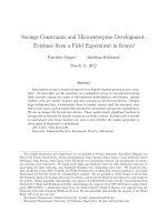
intervention.
24

The coefficient on assignment to the commitment-
treatment group (␤
T1
of equation (2) from Section III) of P235 is
positive and significant at the 90 percent level (Table VI, column
(1)). This estimate corresponds to a 47 percent increase in savings
for the commitment treatment group relative to the control group
(Table II shows baseline savings of P503 for the treatment group).
After twelve months the coefficient estimate is P411—positive
and significant at the 90 percent level (Table VI, column (3)),
which corresponds to an 82 percent increase in savings for the
commitment treatment group relative to the control. The market-
ing effect, denoted by the coefficient on the second treatment
group, ␤
T2
, is insignificant in both intervention periods. The
estimate for ␤
T1
Ϫ␤
T2
(the differential effect of being offered the
commitment savings product beyond being offered only a market-
ing treatment) is positive, but it is statistically indistinguishable
from zero. We repeat the estimation of equation (2) using only the
clients in the treatment and marketing groups. Hence, here the
marketing group (rather than the control group) serves as the
comparison for the treatment group. The estimate of the commit-
ment treatment effect is positive, but statistically insignificant in
both the six- and twelve-month intervention periods (Table VI,
columns (2) and (4)). The regressions in Table VI are repeated

while controlling for a host of demographic and financial vari-
ables. The qualitative results change little after controlling for
these variables. Impact estimates are also robust to regressing
postintervention savings level on treatment assignment, control-
ling for preintervention savings level. Appendix 2 reports these
results. The statistical insignificance masks the heterogeneity in
the impact of the commitment treatment relative to the market-
ing treatment throughout the distribution of the change in bal-
ance variable. Using measures that minimize the influence of
outliers, e.g., the probability of a savings increase and the quan-
tile regressions below, we find a significant commitment-treat-
ment effect relative to the marketing treatment.
First, we generate two binary outcome variables: the first is
24. Change in savings was chosen as the outcome of interest in equation (2)
so that coefficient estimates have the interpretation of average increase in savings
due to the treatment assignment. The results are similar when postintervention
savings level is used as the outcome variable, or when pre- and postintervention
savings data are pooled in a differences-in-differences approach. Appendix 2
reports robustness checks of the ITT analysis. Columns (5)–(6) report ITT esti-
mates where postintervention savings level is regressed against treatment as-
signment and a control for preintervention savings level. ITT estimates change
little relative to estimates reported in Table VI.
658 QUARTERLY JOURNAL OF ECONOMICS
TABLE VI
IMPACT ON CHANGE IN SAVINGS HELD AT BANK
OLS, PROBIT
INTENT TO
TREAT EFFECT OLS Probit
Length 6 months 12 months 12 months
Dependent

variable:
Change in
total
balance
Change in
total
balance
Change in
total
balance
Change in
total
balance
Binary outcome
ϭ 1 if change
in balance Ͼ
0%
Binary outcome
ϭ 1 if change
in balance Ͼ
0%
Binary outcome
ϭ 1 if change
in balance Ͼ
20%
Binary outcome
ϭ 1 if change
in balance Ͼ
20%
Sample All (1)

Commitment &
marketing only
(2)
All (3)
Commitment &
marketing only
(4)
All (5)
Commitment &
marketing only
(6)
All (7)
Commitment &
marketing only
(8)
Commitment
treatment
234.678* 49.828 411.466* 287.575 0.102*** 0.056** 0.101*** 0.064***
(101.748) (156.027) (244.021) (228.523) (3.82) (0.026) (0.022) (0.021)
Marketing
treatment
184.851 123.891 0.048 0.041
(146.982) (153.440) (1.56) (0.027)
Constant 40.626 225.476* 65.183 189.074**
(61.676) (133.405) (124.215) (90.072)
Observations 1777 1308 1777 1308 1777 1308 1777 1308
R
2
0.00 0.00 0.00 0.00
Robust standard errors are in parentheses. * significant at 10 percent; ** significant at 5 percent; *** significant at 1 percent. The dependent variable in the first two columns is the

change in total savings held at the Green Bank after six months. Column (1) regresses change in total savings balances on indicators for assignment in the commitment- and
marketing-treatment groups. The omitted group indicator in this regression corresponds to the control group. Column (2) shows the regression restricting the sample to commitment-
and marketing-treatment groups. Columns (3) and (4) repeat this regression, using change in savings balances after twelve months as a dependent variable. The dependent variable in
columns (5)–(8) is a binary variable equal to 1 if balances increased by x percent. One hundred and fifty-four clients had a preintervention savings balance equal to zero. Twenty-four
of them had positive savings after twelve months. These individuals were coded as “one,” and those that remain at zero were coded as zero for the outcome variables for columns (5)
through (8). Exchange rate is 50 pesos for U.S. $1.
659TYING ODYSSEUS TO THE MAST