Interest Rate Forecasts: A Pathology∗ docx

Interest Rate Forecasts: A Pathology
∗
Charles A. E. Goodhart and Wen Bin Lim
Financial Markets Group
London School of Economics
This paper examines how well forecasters can predict the
future time path of (policy-determined) short-term interest
rates. Most prior work has been done using U.S. data; in
this exercise we use forecasts made for New Zealand by the
Reserve Bank of New Zealand (RBNZ) and those derived from
money market yield curves in the United Kingdom. We broadly
replicate recent U.S. findings for New Zealand and the United
Kingdom, to show that such forecasts in New Zealand and
the United Kingdom have been excellent for the immediate
forthcoming quarter, reasonable for the next quarter, and use-
less thereafter. Moreover, when ex post errors are assessed
depending on whether interest rates have been in an upward,
or downward, section of the cycle, they are shown to have been
biased and, apparently, inefficient. We attempt to explain those
findings, and examine whether the apparent ex post forecast
inefficiencies may still be consistent with ex ante forecast effi-
ciency. We conclude, first, that the best forecast may be a
hybrid containing a specific forecast for the next six months
and a “no-change” assumption thereafter, and, second, that
the modal forecast for interest rates, and maybe for other vari-
ables as well, is skewed, generally underestimating the likely
continuation of the current phase of the cycle.
JEL Codes: C53, E17, E43, E47.
1. Introduction
The short-term policy interest rate has generally been adjusted in
most developed countries, at least during the last twenty years or so,

in a series of small steps in the same direction, followed by a pause
∗
Author contact: C.A.E. Goodhart, Financial Markets Group, Room R414,
London School of Economics, Houghton Street, London WC2A 2AE, United
Kingdom. E-mail:
135
136 International Journal of Central Banking June 2011
Figure 1. Official Cash Rate: Reserve Bank of
New Zealand
Source: Reserve Bank of New Zealand.
and then a, roughly, similar series of steps in the opposite direction.
Figures 1 and 2 show the time path of policy rates for New Zealand
and the United Kingdom, respectively.
On the face of it, such a behavioral pattern would appear quite
easy to predict. Moreover, central bank behavior has typically been
modeled by fitting a Taylor reaction function incorporating a lagged
dependent variable with a large (often around 0.8 at a quarterly peri-
odicity) and highly significant coefficient. But if this was, indeed, the
reason for such gradualism, then the series of small steps should be
highly predictable in advance.
The problem is that the evidence shows that they are not well
predicted, beyond the next few months. There is a large body of,
mainly American, literature to this effect, with the prime exponent
being Glenn Rudebusch with a variety of co-authors; see in particular
Rudebusch (1995, 2002, and 2006). Indeed, prior to the mid-1990s,
there is some evidence that the market could hardly predict the
likely path, or direction of movement, of policy rates over the next
few months in the United States (see Rudebusch 1995 and 2002
and the literature cited there). More recently, with central banks
having become much more transparent about their thinking, their

Vol. 7 No. 2 Interest Rate Forecasts: A Pathology 137
Figure 2. Official Bank Rate: Bank of England
Source: Bank of England web site.
plans, and their intentions, market forecasts of the future path of
policy rates have become quite good over the immediately forthcom-
ing quarter, and better than a random-walk (no-change) assumption
over the following quarter. But thereafter they remain as bad as ever
(see Lange, Sack, and Whitesell 2003 and Rudebusch 2006).
We contribute to this literature first by extending the empiri-
cal analysis to New Zealand and the United Kingdom, though some
similar work on UK data has already been done by Lildholdt and
Wetherilt (2004). The work on New Zealand is particularly interest-
ing, since the forecasts are not those derived from the money market
but those made available by the Reserve Bank of New Zealand in
their Monetary Policy Statements about their current expectations
for their own future policies.
One of the issues relating to the question of whether a central
bank should attempt to decide upon, and then publish, a prospec-
tive future path for its own policy rate, as contrasted with relying
on the expected path implicit in the money market yield curve, is
the relative precision of the two sets of forecasts. A discussion of
the general issues involved is provided by Goodhart (2009). For an
analytical discussion of the effects of the relative forecasting pre-
cision on that decision, see Morris and Shin (2002) and Svensson
138 International Journal of Central Banking June 2011
(2006). An assessment of the effects of publicly announcing the fore-
cast on market rates is given in Andersson and Hofmann (2009) and
in Ferrero and Nobili (2009).
The question of the likely precision of a central bank’s forecast
of its own short-run policy rate is, however, at least in some large

part, empirical. The Reserve Bank of New Zealand (RBNZ), a serial
innovator in so many aspects of central banking, including inflation
targeting and the transparency (plus sanctions) approach to bank
regulation, was, once again, the first to provide a forecast of the
(conditional) path of its own future policy rates. It began to do
so in 2000:Q1. That gives twenty-eight observations between that
date and 2006:Q4, our sample period. While still short, this is now
long enough to undertake some preliminary tests to examine forecast
precision.
Partly for the sake of comparison,
1
we also explore the accuracy
of the implicit market forecasts of the path of future short-term
interest rates in the United Kingdom. We use estimates provided by
the Bank of England over the period 1992:Q4 until 2004:Q4. There
are two such series, one derived from the London Interbank Offered
Rate (LIBOR) yield curve and one from short-dated government
debt. We base our choice between these on the relative accuracy of
their forecasts. On this basis, as described in section 3, we chose,
and subsequently used, the government debt series and its implied
forecasts.
In the next section, section 2, we report and describe our data
series. Then in section 3 of this paper we examine the predictive
accuracy of these sets of interest rate forecasts. The results are
closely in accord with the earlier findings in the United States.
1
The United Kingdom and New Zealand (NZ) are different economies, and
so one is not strictly comparing like with like. If one was, however, to compare
the NZ implicit market forecast accuracy with that of the RBNZ forecast over
the same period (a comparison which we hope that the RBNZ will do), the for-

mer will obviously be affected by the latter (and possibly vice versa). Again, if a
researcher was to compare the implied accuracy of the market forecast prior to
the introduction of the official forecast with the accuracy of the market/official
forecast after the RBNZ had started to publish (another exercise that we hope
that the RBNZ will undertake), then the NZ economy, their financial system, and
the economic context may have changed over time. So one can never compare an
implicit market forecast with an official forecast for interest rates on an exactly
like-for-like basis. Be that as it may, we view the comparison of the RBNZ and the
implied UK interest rate forecasts as illustrative, and not definitive in any way.
Vol. 7 No. 2 Interest Rate Forecasts: A Pathology 139
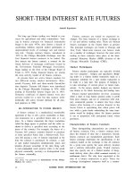
Figure 3. RBNZ Interest Rate Forecast (Ninety Days,
Annualized Rate) Published in Successive Monetary
Policy Statements
Notes: Turning points are marked by a diamond. The dating of these is discussed
further in section 3.
Whether the forecast comes from the central bank or from the mar-
ket, the predictive ability is good, by most econometric standards,
over the first quarter following the date of the forecast; it is poor, but
significantly better than a no-change, random-walk forecast, over the
second quarter (from end-month 3 to end-month 6), and effectively
useless from that horizon onward.
Worse, however, is to come. The forecasts, once beyond the end
of the first quarter, are not only without value, they are, when com-
pared with ex post outcomes, also strongly and significantly biased.
This does not, however, necessarily mean that the forecasts were ex
ante inefficient. We shall demonstrate in section 5 how ex post bias
can yet be consistent with ex ante efficiency in forecasting.
This bias can actually be seen clearly in a visual representation of
the forecasts. The RBNZ forecasts and outcome are shown in figure
3, and the UK forecast derived from the short-dated government

debt yield curve and outcome is shown in figure 4.
What is apparent by simple inspection is that when interest rates
are on an upward (downward) cyclical path, the forecast underesti-
mates (overestimates) the actual subsequent path of interest rates.
Much the same pattern is also observable in the United States (see
140 International Journal of Central Banking June 2011
Figure 4. UK Interest Rate Forecast (Ninety Days,
Annualized Rate) Derived from the Short-Dated
Government Debt Yield Curve
Rudebusch 2007) and Sweden (see Adolfson et al. 2007). One of the
reasons why this bias has not been more widely recognized up till
now is that the biases during up and down cyclical periods are almost
exactly offsetting, so if an econometrician applies his or her tests
to the complete time series (as usual) (s)he will find no aggregate
sign of bias. The distinction between the bias in “up” and “down”
periods is crucial. A problem with some time series—e.g., those for
inflation—is that the division of the sample into “up,” “down,” and
in some cases “flat” periods is not always easy, nor self-evident. But
this is less so for short-term interest rates where the ex post timing
of turning points is relatively easier.
The sequencing of this paper proceeds as follows. We report our
database in section 2. We examine the accuracy of the interest rate
forecasts in section 3. We continue in section 4 by assessing whether
forecasts which appear ex post biased can still be ex ante efficient.
Section 5 concludes.
2. The Database for Interest Rates
Our focus in this paper concerns the accuracy of forecasts for short-
term policy-determined interest rates, measured in terms of unbi-
asedness and the magnitude of forecast error. We examine the data
for two countries. We do so first for New Zealand, because this is the

Vol. 7 No. 2 Interest Rate Forecasts: A Pathology 141
country with the longest available published series of official projec-
tions, as presented by the RBNZ in their quarterly Monetary Policy
Statement. Our second country is the United Kingdom. In this case
the Bank of England assumed unchanged future interests, from their
current level, as the basis of their forecasts, until they moved onto a
market-based estimate of future policy rates in November 2004. As
described below, we considered the use of two alternative estimates
of future (forecast) policy rates.
In New Zealand, policy announcements, and the release of pro-
jections, are usually made early in the final month of the calendar
quarter, though the research work and discussions in their Monetary
Policy Committee (MPC) will have mostly taken place a couple of
weeks previously. Thus the Statement contains a forecast for infla-
tion for the current quarter (h = 0), though that will have been made
with knowledge of the outturn for the first month and some partial
evidence for the second. The Policy Targets Agreement between the
Treasurer and the Governor is specified in terms of the CPI, and
the forecast is made in terms of the CPI. This does not, however,
mean that the RBNZ focuses exclusively on the overall CPI in its
assessment of inflationary pressures.
In New Zealand, the policy-determined rate is taken to be the
ninety-day (three-month) rate, and the forecasts are for that rate.
Thus the current-quarter interest rate observation contains nearly
two months of actual ninety-day rates and just over one month of
market forward one-month rates. If the MPC meeting results in a
(revisable) decision to change interest rates in a way that is incon-
sistent with the prediction that was previously embedded in market
forward interest rates, then the assumption for the current quarter
can be revised to make the overall ninety-day track look consistent

with the policy message. Finally, the policy interest rate can be
adjusted, after the forecast is effectively completed, right up to the
day before the Monetary Policy Statement; this was done in Septem-
ber 2001 after the terrorist attack. So, the interest rate forecast for
the current quarter (h = 0) also contains a small extent of uncertain
forecast.
The data for published official forecasts of the policy rate start
in 2000:Q1. We show those data, the forecasts, and the resulting
errors, for the policy rate in the appendix, tables 8 and 9. The data
are shown in a format where the forecasts are shown in the same
142 International Journal of Central Banking June 2011
row as the actual to be forecast, so the forecast errors can be read
off directly.
The British case is somewhat more complicated. In the past,
during the years of our sample, the MPC used a constant forward
forecast of the repo rate as the conditioning assumption for its fore-
casting exercise. Whether members of the MPC made any mental
reservations about the forecast on account of a different subjective
view about the future path of policy rates is an individual question
that only they can answer personally. But it is hard to treat that
constant path as a pure, most likely, forecast. At the same time,
there are at least two alternative time series of implied market fore-
casts for future policy rates that are derived from the yield curve of
short-dated government debt and from LIBOR. There are some com-
plicated technical issues in extracting implied forecasts from market
yield curves, and such yield curves can be distorted, especially the
LIBOR yield curve, as experience since 2007 has clearly demon-
strated. These problems relate largely to risk premia, notably credit
and default risk; see Ferrero and Nobili (2009). The yield curve for
government debt is (or rather has been) largely immune to such

credit (default) risk, though it can be exposed to other risks, e.g.,
interest rate and liquidity risks.
We do not rehearse these difficulties here; instead we simply
took these data from the Bank of England web site (see www.
bankofengland.co.uk). For more information on the procedures used
to obtain such implicit forecast series, see Anderson and Sleath
(1999, 2001), Brooke, Cooper, and Scholtes (2000), and Joyce,
Relleen, and Sorensen (2007). As will be reported in the next section,
the government debt implicit market forecast series has had a more
accurate forecast than the LIBOR series over our data period, 1992–
2004, probably in part because the government series would not
have incorporated a time-varying credit risk element; see Ferrero and
Nobili (2009). Since the constant rate assumption was hardly a fore-
cast, most of our work was done with the government debt implicit
forecast series. This forecasts the three-month Treasury bill series.
These series—actual, forecast, and errors (with the forecast lined up
against the actual it was predicting)—are shown in the appendix,
tables 10 and 11, for the government debt series (the other series for
LIBOR is available from the authors on request).
Vol. 7 No. 2 Interest Rate Forecasts: A Pathology 143
3. How Accurate Are the Interest Rate Forecasts?
We began our examination of this question by running three regres-
sions both for the NZ data series and for two sets of implied market
forecasts for the United Kingdom, derived from the LIBOR and gov-
ernment debt yield curve, respectively. These regression equations
were as follows:
IR(t + h)=C
1
+ C
2

Forecast (t, t + h) (1)
IR(t + h) − IR(t)=C
1
+ C
2
[Forecast(t, t + h) − IR(t)]
(2)
IR(t + h) − IR(t + h − 1) = C
1
+ C
2
[Forecast(t, t + h)
− Forecast(t, t + h − 1)], (3)
where
IR(t) = actual interest rate outturn at time t
Forecast(t, t + h) = forecast of IR(t + h) made at time t.
The first equation is essentially a Mincer-Zarnowitz regression
(Mincer and Zarnowitz 1969) evaluating how well the forecast can
predict the actual h-period-ahead interest rate outturn (h =0to
n). If the forecast perfectly matches the actual interest rate out-
turn for every single period, we would expect to have C
2
= 1 and
C
1
= 0. This can be seen as an evaluation of the bias of the fore-
cast. Taking expectations on both sides, E{IR(t + h)} = E{C
1
+
C

2
[Forecast(t, t + h)}. A forecast is unbiased—i.e., E{IR(t + h)} =
E{[Forecast(t, t + h)]} for all t—if and only if C
2
= 1 and C
1
=0.
The second regression, by subtracting the interest rate level from
both sides, allows us to focus our attention on the performance of
the forecast interest rate difference {IR(t + h) − IR(t)}. It asks, as
h increases, how accurately can the forecaster forecast h-quarter-
ahead interest rate changes from the present level. The third regres-
sion is a slight twist on the second, focusing on one-period-ahead
forecasts; the regression examines the forecast performance of one-
period-ahead interest rate changes {IR(t + h) − IR(t + h − 1)} as h
increases.
144 International Journal of Central Banking June 2011
All three regressions assess the accuracy/biasness of interest rate
forecasts from slightly different angles. An unbiased forecast nec-
essarily implies a constant term of zero and a slope coefficient of
one. We can test whether these conditions are fulfilled with a joint
hypothesis test:
H
0
: C
1
= 0 and C
2
=1.
With three equations, three data sets, and h = 0 to 5 for New

Zealand and h = 1 to 8 for the UK series, we have some eighty-five
regression results and statistical test scores to report.
We found that the regression results, estimated by OLS, for the
implicit forecasts derived from the LIBOR yield curve were compre-
hensively worse than those from the government yield curve, or the
RBNZ. These LIBOR results provided poor forecasts even for the
first two quarters, and useless forecasts thereafter. There are several
possible reasons for such worse forecasts—e.g., time-varying risk pre-
mia (Ferrero and Nobili 2009) or data errors in a short sample—but
it is beyond the scope of this paper to try to track them down. These
results can be found in Goodhart and Lim (2008) and, to save space,
are not reported here. That reduces the number of regression results
to sixteen in table 1 for the RBNZ and twenty-four in table 2 for the
UK government yield curve.
These results show that the RBNZ forecast is excellent one quar-
ter ahead but then becomes useless in forecasting the subsequent
direction, or extent, of change. Thus the coefficient C
2
in equation
(3) becomes −0.04 at h = 2 (with an R-squared of zero), and neg-
ative thereafter. When the equation is run in levels, rather than
first differences—i.e., equation (1)—the excellent first-quarter fore-
cast feeds through into a significantly positive forecast of the level
in the next few quarters, though it is just the first-quarter forecast
doing all the work. The Mincer-Zarnowitz test results
2
are also con-
sistent with our findings. We failed to reject the joint hypothesis H
0
for up to a three-quarters-ahead forecast for equation (1) and up to

a four-quarters-ahead forecast for equation (2). We reject H
0
for the
quarters thereafter.
2
These tests are reported in Goodhart and Lim (2008) but are omitted to save
space here.
Vol. 7 No. 2 Interest Rate Forecasts: A Pathology 145
Table 1. Regression Results for New Zealand
C
1
C
2
h = (p-value) (p-value) R-squared DW
Equation (1)
0 −0.01 1.00 0.99 1.77
(0.93) (0.85)
1 −0.24 1.03 0.88 1.53
(0.64) (0.74)
2 0.30 0.93 0.65 0.93
(0.75) (0.63)
3 1.50 0.74 0.39 0.34
(0.25) (0.19)
4 3.71 0.40 0.11 0.28
(0.03) (0.02)
5
5.71 0.09 0.00 0.15
(0.00) (0.00)
Equation (2)
1 −0.16 1.61 0.35 1.61

(0.07) (0.18)
2 −0.15
1.02 0.20 1.02
(0.31) (0.95)
3 −0.09 0.73 0.10 0.45
(0.66) (0.55)
4
0.13 0.11 0.00 0.47
(0.61) (0.10)
5 0.37 −0.38 0.03 0.34
(0.20) (0.01)
Equation (3)
1 0.13 1.30 0.43 2.06
(0.07) (0.33)
2 0.04 −0.04 0.00 1.24
(0.65) (0.06)
3 0.07 −0.68 0.03 1.38
(0.38) (0.04)
4 0.09 −1.29 0.07 1.37
(0.28) (0.03)
5 0.09 −1.30 0.08 1.28
(0.26) (0.02)
Note: The corresponding p-value is evaluated against the null hypothesis,
H
0
: C
1
=0,C
2
=1.

146 International Journal of Central Banking June 2011
Table 2. UK Forecasts Derived from the Short-Term
Government Yield Curve
C
1
C
2
h = (p-value) (p-value) R-squared DW
Equation (1)
1 0.23 0.98 0.95 1.94
(0.25) (0.64)
2 0.60 0.89 0.84 1.03
(0.07) (0.06)
3 0.98 0.79 0.71 0.62
(0.03) (0.01)
4 1.56 0.67 0.55 0.43
(0.00) (0.00)
5 2.10 0.56 0.41 0.35
(0.00) (0.00)
6 2.43 0.49 0.34 0.31
(0.00) (0.00)
7 2.52 0.47 0.32 0.29
(0.00) (0.00)
8
2.42 0.48 0.35 0.28
(0.00) (0.00)
Equation (2)
1 0.13 0.94 0.51 1.91
(0.02)
(0.70)

2 −0.01 0.86 0.50 1.04
(0.84) (0.31)
3 −0.16 0.85 0.47 0.67
(0.09) (0.25)
4 −0.28 0.73 0.36 0.48
(0.03) (0.07)
5 −0.34 0.60 0.27 0.39
(0.03) (0.01)
6 −0.37 0.51 0.22 0.35
(0.03) (0.00)
7 −0.39 0.46 0.21 0.31
(0.02) (0.00)
8 −0.43 0.46 0.24 0.28
(0.00) (0.00)
(continued)
Vol. 7 No. 2 Interest Rate Forecasts: A Pathology 147
Table 2. (Continued)
C
1
C
2
h = (p-value) (p-value) R-squared DW
Equation (3)
1 0.13 0.94 0.51 1.91
(0.02) (0.70)
2 −0.13 0.87 0.25 1.19
(0.02) (0.62)
3 −0.13
0.65 0.15 0.97
(0.04) (0.14)

4 −0.09 0.43 0.05 0.83
(0.19) (0.03)
5 −0.08 0.53 0.06 0.84
(0.21) (0.14)
6 −0.08 0.73 0.08 0.80
(0.18) (0.15)
7 −0.06 0.41 0.04
0.82
(0.34) (0.58)
8 −0.05 0.58 0.03 0.76
(0.39) (0.41)
Note: The corresp onding p-value is evaluated against the null hypothesis, H
0
:
C
1
=0,C
2
=1.
Turning next to the United Kingdom implied forecasts from the
government debt yield curve, what these tables indicate is that, in
the first quarter after the forecast is made, the forecast precision
of this derived forecast is mediocre (joint test for null hypothe-
sis is rejected for h =3− 8), certainly significantly better than
random walk (no change) but not nearly as good as the NZ fore-
cast over its first quarter. However, this market-based forecast is
also able to make a good forecast of the change in rates between
Q1 and Q2 (whereas the RBNZ could not do that). The govern-
ment yield forecast for h = 2 in table 2 is somewhat better than
for h = 1. So the ability of the government yield forecast to pre-

dict the level of the policy rate two quarters (six months) hence
is about the same or a little better than that of the RBNZ. There-
after, from Q2 onward, the predictive ability of the government yield
148 International Journal of Central Banking June 2011
Figure 5. Stylized Pattern of Relationships between
Forecasts and Outturns of Macro Variables over the Cycle
forecast becomes insignificantly different from zero, but at least the
coefficients have the right sign (unlike the RBNZ).
The conclusion of this set of tests is that the precision of inter-
est forecasts beyond the next quarter or two is approximately zero,
whether they are made by the RBNZ or the UK market. Given the
gradual adjustments in actual policy rates, this might seem surpris-
ing. Why does it happen? In order to answer this question, we start
with a stylized fact. When one looks at most macroeconomic fore-
casts, and notably so for interest rates (see figures 3 and 4 above),
they tend to follow a pattern. When the macro variable is rising,
the forecast increasingly falls below it. When the macro variable is
falling, the forecast increasingly lies above it. This pattern is shown
again in illustrative form in figure 5.
So, if we divide the sample period into periods of rising and
falling values for the variable of concern (in this case the interest
rate), during up periods Actual minus Forecast will tend to be per-
sistently positive, and during down periods Actual minus Forecast
will tend to be persistently negative. There is, however, an impor-
tant caveat. A forecast made during an up (down) period may extend
several quarters beyond the turning point into the next down (up)
period. Once a turning point has occurred, however, a forecast that
was too high (low) during the continuing down (up) cycle can rapidly
then become too low (high) once the cycle has switched direction.
Clearly the tendency for Actual minus Forecast to be negative in

an upturn will be most marked for forecasts made in an upturn so
long as that upturn continues, i.e., until the next sign change from
Vol. 7 No. 2 Interest Rate Forecasts: A Pathology 149
up to down, or vice versa. Nevertheless, we still expect on balance
that forecasts made during an upturn (downturn) will tend to have
positive (negative) Actual minus Forecast outturns even after such
a sign change, but the result is clearly uncertain.
3
But the forecasts
made for the policy rate in the next quarter (and to a lesser extent
into the second quarter) are so good, especially for the next quarter
for the RBNZ, that no such bias may exist.
As can be seen from figures 1 and 2, the official rate is frequently
held constant for a period of a few months before there is a reversal
of direction. So the exact date of reversal is somewhat uncertain.
We chose a date during these months as the best alternative on the
basis of other available contemporaneous evidence, notably the con-
current time path of market rates. But we also tested for robustness
by taking the first and last dates of each flat period and rerunning
the exercises. The latter made no difference; the results are available
on request from the authors.
Perhaps the easiest way of demonstrating this result, suggested
to us by Andrew Patton, is to run a regression of the forecast error, at
various horizons, against two indicator variables, one for up periods
(C
1
) and one for down periods (C
2
):
4

[IR(t + h) − Forecast(t, t + h)] = C
1
I
up
(t + h)+C
2
I
down
(t + h),
(4)
where
IR(t) = actual interest rate outturn at time t
Forecast(t, t + h) = forecast of IR(t + h) made at time t
I
up
(t + h) is a dummy variable = 1 if time,t+ h,
is an “up” period; else 0
I
down
(t + h) is a dummy variable = 1 if time,t+ h,
is a “down” period; else 0.
3
When interest rates are volatile, and sign changes are more frequent, nothing
useful can be said about the likely outcomes of Actual minus Forecast after a
second sign change.
4
In our original paper (Goodhart and Lim 2008), we did some additional and
more complicated statistical exercises, looking at the number of errors of a par-
ticular sign, in “up” and “down” phases, their mean, standard deviation, and
p-values. They are omitted here to save space.

150 International Journal of Central Banking June 2011
Table 3. Results for New Zealand
A. Indicator Variable Is Based on State in NZ at
Outturn Date (Whole Data Set)
H = Adj. R-sqr. C
1
p-value C
2
p-value
Q1 0.41 0.06 0.26 −0.34 0.00
Q2 0.61 0.14 0.07 −0.69 0.00
Q3 0.58 0.23 0.06 −0.88 0.00
Q4 0.36 0.23 0.23 −0.99 0.00
Q5 0.27 0.24 0.33 −1.06 0.01
Q6 0.20 0.23 0.49 −1.07 0.05
Q7 0.03 0.13 0.79 −0.95 0.27
Q8 −0.30 0.04 0.97 −0.52 0.79
B. Indicator Variable Is Based on State in NZ at
Outturn Date, but only Includes Period during
Which Sign Is Unchanged
H = Adj. R-sqr. C
1
p-value C
2
p-value
Q1 0.41 0.06 0.26 −0.34 0.00
Q2 0.76 0.22 0.00 −0.70 0.00
Q3 0.87 0.41 0.00 −1.13 0.00
Q4 0.81 0.56 0.00 −1.53 0.00
Q5 0.86 0.73 0.00 −2.13 0.00

Q6 — — — — —
Q7 — — — — —
Q8 — — — — —
Note: The corresp onding p-value is evaluated against the null hypothesis, H
0
:
C
1
=0,C
2
=0.
The hypothesis is that the up-period indicator (C
1
) is positive
(actual > forecast) and the down-period indicator (C
2
) is negative
(actual < forecast).
The results for New Zealand are shown in table 3.
Turning next to the results for the UK government yield implied
forecasts, we found similar results. In this case, however, the
forecasts included some sizable average errors, whereby the fore-
casts implied that interest rates would tend to become higher than
was the case in the historical event (actual < forecast). This average
Vol. 7 No. 2 Interest Rate Forecasts: A Pathology 151
Figure 6. Average UK Interest Rate Forecast Error
error tended to increase, approximately linearly, as the horizon (h)
increased. This is shown in figure 6.
After correcting for this average error
5

and rerunning,
6
the
results were as shown in table 4.
One of our referees kindly directed our attention to a related
recent article, Ferrero and Nobili (2009). In this they regress excess
returns (x), defined as forecast less actual ex post outcomes, for
interest rates (futures) as a function of a business-cycle indicator
(growth of output or employment expectations) and the current level
of the futures rate, so that in their equation (4), p. 116,
x
(n)
t+n
= a
(n)
+ β
n
z
t
+ γ
n
f
(n)
t
+ ε
(n)
t+n
,
where z
t

is the business-cycle indicator, f
t
is the level of the current
futures rate, and β and γ are coefficients. In their table 2 (p. 118),
table 5 (p. 127), and table 7 (p. 131), they find β to be negative,
often significantly so, and γ to be usually significantly positive.
These authors cannot explain their own findings: “A theoretical
analysis of the reasons behind the presence of forecast errors that
are predictable and significantly countercyclical only in the United
5
The tables using the unadjusted data—i.e., without correcting for the average
error—are available on request from the authors.
6
The average forecast error in New Zealand was much smaller and did not
vary systematically with h. We ran similar adjusted regressions for New Zealand,
but the results were closely similar to those shown in table 4.
152 International Journal of Central Banking June 2011
Table 4. Results for United Kingdom, with Average
Error Removed
A. Indicator Variable Is Based on State in UK at
Outturn Date (Whole Data Set, with Average
Forecast Error Removed)
H = Adj. R-sqr. C
1
p-value C
2
p-value
Q1 0.14 0.12 0.10 −0.08 0.16
Q2 0.25 0.26 0.01 −0.19 0.02
Q3 0.41 0.45 0.00 −0.38 0.00

Q4 0.22 0.41 0.02 −0.39 0.02
Q5 0.07 0.27 0.24 −0.30 0.17
Q6 0.01 0.04 0.89 −0.13 0.60
Q7 0.00 −0.19 0.50 −0.03 0.91
Q8 0.03 −0.40 0.16 0.01 0.97
B. Indicator Variable Is Based on State in UK at
Outturn Date, but only Includes Period during Which Sign
Is Unchanged, with Average Forecast Error Removed
H = Adj. R-sqr. C
1
p-value C
2
p-value
Q1 0.14 0.12 0.10 −0.08 0.16
Q2 0.32 0.28 0.01 −0.25 0.00
Q3 0.63 0.57 0.00 −0.55 0.00
Q4 0.70 0.79 0.00 −0.72 0.00
Q5 0.76 0.85 0.00 −0.88 0.00
Q6 0.81 0.76 0.00 −0.80 0.00
Q7 0.76 0.76 0.03 −0.89 0.00
Q8 0.67 0.52 0.23 −0.95 0.00
States lies beyond the scope of this paper” (Ferrero and Nobili 2009,
p. 130). Our analysis here enables us to explain these findings; they
are exactly what we would have expected given the ex post biases
in forecasting over the cycle phases. As shown illustratively in figure
5, during the up (down) phases of the cycle, forecasts understate
(overstate) ex post actuals systematically; hence β will be negative,
though we too cannot explain why the euro zone exhibits less of this
effect. Similarly, the expected futures rate will tend to be highest
(lowest) at the top (bottom) of the cycle. As figure 5 again shows,

this is when the forecast bias has forecast greater (less) than actual,
so γ should be positive. The explanation of the Ferrero/Nobili results
is, in our view, not due to time-varying risk premia, but to system-
atic ex post biases in the forecasting process over cycle phases. We
Vol. 7 No. 2 Interest Rate Forecasts: A Pathology 153
are particularly grateful for having been given the chance to relate
our work here to another strand in the literature.
What all these results show is as follows:
(i) The official and market forecasts of interest rates that we
have studied here have significant predictive power over the
next two quarters, but virtually none thereafter. When fore-
cast precision is effectively zero, as after two quarters hence,
it is perhaps best to acknowledge this, e.g., by the central
bank using either a “no-change” thereafter assumption, or
the implied market forecast, for the more distant forecasts.
7
(ii) These interest rate forecasts are systematically biased, under-
estimating future policy rates during upturns and overesti-
mating them during downturns. We shall now proceed to
explore reasons why this might have been so in sections 4
and 5.
4. Can One Forecast the Forecasters?
In the preceding sections, we have shown that interest rate forecasts
in the United Kingdom and New Zealand during this time period sys-
tematically underpredicted the time series during cyclical phases of
upward movement, and similarly overpredicted during downswings.
In this section we seek to address the question of why these
(most?) forecasts exhibit this tendency.
8
The answer that we pro-

pose is that (most) macroeconomic variables are expected (by most
7
The choice may depend on the confidence with which the official forecasters
hold their longer-dated forecasts. There is, however, a danger that the official
forecasters have excessive confidence in their own forecasting abilities and that
private-sector forecasters likewise place excessive weight on such official forecasts
(Morris and Shin 2002). However, the finding by Ferrero and Secchi (2009) that
long-term expectations on future interest rates react significantly only to short-
term central bank interest rate forecasts, and not to their longer-term projections,
suggests that market agents may well realize that such longer-term projections
rarely contain any valuable information.
8
In our original work we extended our research to cover inflation forecasts
as well. These also exhibited the same syndrome. In order to save space and
to enhance focus, we have, however, omitted those results from this paper. A
more extended version of this paper, which explores not only the (errors in the)
inflation forecasts in New Zealand and the United Kingdom but also the rela-
tionships between the errors in the inflation forecasts and those in the interest
rate forecasts, is given in Goodhart and Lim (2009).
154 International Journal of Central Banking June 2011
economists
9
) to revert to some longer-term equilibrium, ceteris
paribus. Indeed, it is hard to see how forecasting could be done
in the absence of a concept of (long-run) equilibrium. But at any
particular point of time, macroeconomic variables will be subject to
momentum, whose current force is quite difficult to assess accurately
and which will be subject to unforeseeable future shocks. Thus we
posit that these (most) forecasts will be subject to two main ele-
ments, an autoregressive component and a mean-reverting (back to

equilibrium) component. Such a combination is bound to give us
the general pattern that we have found in practice. So long as the
phase remains upward (downward), the mean-reverting element in
the forecast will tend to pull the forecast below (above) the actual
track of the variable, but, of course, as the eventual turning point
draws closer, it will predict far better than a pure autoregressive
forecast.
During the periods under examination, an inflation-targeting
regime was in operation in both New Zealand and the United
Kingdom, so the equilibrium to which the inflation rate would revert
would have been close to target, and about 2
1
2
percent above that
for the nominal interest rate, assuming an equilibrium real interest
rate of 2
1
2
percent. But for our purposes here, we do not assume to
know what the equilibrium interest rate is, and have simply taken
the arithmetic average of the study period as an estimation of the
“mean-reverting” point.
10
The nature of the autoregressive process
for each series, and the coefficients for combining the autoregres-
sive and the mean-reverting components into an implied forecast
are unknown and for determination. Initially we shall assume that
the forecasters make an efficient, unbiased prediction of both factors.
Thus we estimate for each series
IR(t +1)− IR(t)=B

1
∗ [IR(t) − IR(t − 1)] + B
2
∗ [IR(t) − IR], (5)
9
Not all economists have such expectations. A few, “heterodox,” economists
challenge whether equilibria necessarily exist, notably Paul Davidson and Basil
Moore.
10
We tested this by trying values of the mean-reverting point with +1 percent
and −1 percent of the average, and it made no significant difference to the coef-
ficients for B
1
and B
2
, as well as for the results in table 6 and table 7. These
results are available on request from the authors.
Vol. 7 No. 2 Interest Rate Forecasts: A Pathology 155
Table 5. Estimated Coefficients
Regression
Equation (1) B
1
B
2
Statistics
Adj.
Coef. t-stats p-value Coef. t-stats p-value R-sqr. SE Obs.
UK Interest
Rate 0.66 6.30 0.00 −0.09 −2.54 0.01 0.4175 0.2539 54
NZ Interest

Rate 0.49 4.90 0.00
−0.13 −3.58 0.00 0.3403 0.6326 66
Figure 7. NZ Interest Rate: Comparison between
Outturn, Actual and Implied Forecast
where
IR(t) = actual interest rate outturn at time t
IR = average interest rate outturn over the study period.
The estimated coefficients are shown in table 5, where B
1
can be
understood as the autoregressive coefficient, and B
2
as the mean-
reversion coefficient.
Now we have a simplified model of how forecasts are done. The
next step is to compare it with the actual forecasts. We do this first
diagrammatically. For illustration, we have provided the diagram-
matical comparison for the period between 2000:Q1 and 2002:Q4.
The diagrams, figure 7 for New Zealand and figure 8 for the United
156 International Journal of Central Banking June 2011
Figure 8. UK Interest Rate: Comparison between
Outturn, Actual and Implied Forecast
Kingdom, show quite a close relationship between the actual and
our implied (from our simple model) forecast. Quarters beyond t+1
are estimated recursively.
We then evaluate the implied forecast changes against the actual
forecast changes via regression analysis over the whole study period:
Actual Forecast (t, t + h) − IR(t)
= C
1

+ C
2
[Implied Forecast (t, t + h) − IR(t)
i =1− 8. (6)
The hypothesis is that C
1
= 0 and C
2
= 1. The t-stats for C
2
in
table 6 for New Zealand and table 7 for the United Kingdom relate
to the coefficient’s deviation from unity, not from zero.
But the regressions, and a closer inspection of the diagrams, indi-
cated a systematic problem, separating the implied from the actual
forecast. This was that the “true” coefficient of mean reversion dur-
ing these years was greater than that used by the actual forecasters;
i.e., the implied forecast flattened out near the equilibrium level
faster than the actual forecasters expected. An indicative diagram
for the six-quarters-ahead implied forecast for the UK interest rate
showing this is given in figure 9.
11
11
Similar figures for NZ interest rates and for the UK series, both inflation and
interest rates, are available in Goodhart and Lim (2009).
Vol. 7 No. 2 Interest Rate Forecasts: A Pathology 157
Table 6. NZ Interest Rate: Evaluation of Implied Forecast
and Actual Forecast
C
1

C
2
Regression Statistics
Adj.
h Coef. t-stats p-value Coef. t-stats p-value R-sqr. SE Obs.
1 0.05 1.76 0.09 0.48 −4.99 0.00 0.44 0.10 28
2
0.01 0.14 0.89 0.57 −3.87 0.00 0.48 0.17 28
3 −0.03 −0.41 0.69 0.52 −4.20 0.00 0.43 0.24 28
4 −0.04 −0.40 0.69 0.44 −4.95 0.00 0.35 0.30 28
5
−0.05 −0.44 0.66 0.40 −5.35 0.00 0.30 0.35 28
6 −0.13 −0.81 0.43 0.43 −4.36 0.00 0.33 0.38 21
7 −0.21 −1.02 0.33 0.48 −3.22 0.01 0.38 0.41 14
8 −0.31 −0.91 0.41 0.50 −2.12 0.09 0.36 0.48 7
Table 7. UK Interest Rate: Evaluation of Implied
Forecast and Actual Forecast
C
1
C
2
Regression Statistics
h Coef. t-stats p-value Coef. t-stats p-value R-sqr. SE Obs.
1 −0.16 −5.51 0.00 0.89 −0.93 0.36 0.65 0.17 34
2 −0.03 −0.49 0.63 0.81 −1.33 0.19 0.42 0.39 44
3 0.17 1.96 0.06 0.70 −1.84 0.07 0.28 0.59 47
4 0.31 2.82 0.01 0.59 −2.42 0.02 0.20 0.75 47
5 0.43 3.27 0.00 0.50 −2.92 0.01 0.14 0.89 47
6 0.51 3.52 0.00 0.44 −3.33 0.00 0.11 0.99 47
7 0.58 3.66 0.00 0.40 −3.64 0.00 0.09 1.07 47

8 0.63 3.74 0.00 0.37 −3.86 0.00 0.08 1.14 47
Incidentally, the implied forecasts often did better in predicting
the outturns than the actual forecasts. The results are available from
the authors on request. This is not, however, so surprising since the
implied forecasts are obtained by finding the coefficients that best
explained the ex post outturns, i.e., data mining. So we place no
emphasis on this finding.
The actual forecasters placed less weight on mean reversion than
appeared to be the case in our constructed implied forecasts. That
158 International Journal of Central Banking June 2011
Figure 9. UK Interest Rate, Six-Quarters-Ahead Forecast
forecasters should have underestimated the speed of reversion to
the mean is itself both plausible and understandable during these
years. This was, after all, the period of the Great Moderation. A
possible definition of such a Great Moderation is a period when the
key macroeconomic time series revert to their (desired) equilibrium
somewhat faster than in the past or than currently expected.
Most macro variables are cyclical, but, as any forecaster knows
only too well, it is extraordinarily difficult to predict turning points.
Hence a forecast which combines a weighted average of autoregres-
sive continuation and mean reversion is likely to be optimal. It should
minimize the likelihood of a really big error, and will be unbiased
over the medium and longer run. So the behavior of the forecasters
in seeking to estimate the likely mean outturn is, we would argue,
appropriate.
Where our findings do indicate that there is a need for improve-
ment is with the fan chart, or probability distribution, of future
outcomes. This is usually shown as a symmetric single-peaked dis-
tribution, often akin to a normal distribution with mode, mean, and
median at the same point.

Our results show that this will generally not be the case. The
most probable outcome is that the cyclical phase will continue.
Hence in an upturn (downturn), the most probable outcome is that
(inflation and) interest rates will turn out to be systematically above
(below) the mean forecast. But this is balanced by a smaller proba-
bility that the cycle will turn within this interval. But if there should
be such a turning point, following an upturn (downturn) phase, then
Vol. 7 No. 2 Interest Rate Forecasts: A Pathology 159
the forecasts will considerably overstate (understate) the subsequent
downward (upward) movement.
5. Conclusions
In this paper we have demonstrated that, in the two countries and
short data periods studied, the forecasts of interest rates had little
or no informational value when the horizon exceeded two quarters
(six months), though they were good in the next quarter and rea-
sonable in the second quarter out. Moreover, all the forecasts were
ex post and, systematically, inefficient, underestimating (overesti-
mating) future outturns during up (down) cycle phases. The main
reason for this is that forecasters cannot predict the timing of cycli-
cal turning points, and hence predict future developments as a con-
vex combination of autoregressive momentum and a reversion to
equilibrium.
There are, perhaps, two main conclusions that can be drawn from
this. The first is that official interest rate forecasts should probably
be presented in hybrid form. MPCs and markets can make reason-
able forecasts of interest rates up to two (at an extreme pinch,
three) quarters hence. These should, indeed, be the basis of fore-
casts. Beyond that horizon, they are rarely able to do so, and that
too should be acknowledged. Unless the authorities have a particular
reason for exhibiting confidence in their own longer-dated forecasts,

those same (longer-dated) forecasts should be presented in a specif-
ically formulaic manner, e.g., constant or based on implied forward
market rates.
The second conclusion is that the resulting interest (and infla-
tion) forecast is generally not modal. It is biased, underestimating
(overestimating) in upturns (downturns), because the forecaster is
protecting himself or herself against extreme errors by assuming a
(roughly constant) small probability of a turning point in the cycle
occurring in each quarter. Consequently the most likely outturn in
any expansionary phase is that output, inflation, and interest rates
will turn out above forecast (vice versa in a downturn). The con-
clusion that we would draw from this is that policy needs to be
normally somewhat more aggressive than the mean forecast would
indicate (raising rates in booms, cutting rates in recessions), but that
the policymakers need to be alert to (unpredictable) turning points
and therefore to the occasional need to reverse course abruptly.