URBAN AIR POLLUTION: AN ANALYSIS OF THE ENVIRONMENTAL KUZNETS CURVE IN ASIAN CITIES docx

1"|"P age"
%
A Thesis Paper
On the








URBAN AIR POLLUTION:
AN ANALYSIS OF THE
ENVIRONMENTAL KUZNETS CURVE
IN ASIAN CITIES






Submitted by:
GATDULA, Valerie B.
TOLENTINO, Richmay Anne C.




To:
Dr. Rosalina Tan

Professor








In partial fulfillment of the
requirements in
Economics 171: Economics Research I








February 2011
2"|"P age"
%
INTRODUCTION
A. Background of the Problem
Sustainable development has been one of the alarming concerns in the twenty-first
century. Anderson and Brooks (1996) discus how given the fact that “the supply of most
natural resources and environment services” are limited, it is of urgent concern to monitor
and control resource usage for one to even hope for continued economic activity in the years
to come. Furthermore, the incessant population and per capita growth exacerbates the

problem as they are indicative of the continuous growth in economic activity (Anderson &
Brooks, 1996).
Sustainable development has significant implications on the extent of economic
activity in the future. Anderson and Brooks (1996) elaborate saying, “scientific basis
supporting the relationship between business activity, resource depletion and the environment
has grown stronger in recent years.”After all, economic activity is limited and defined by the
state of the environment in which businesses operate, get raw materials from, etc.
The call for sustainable development has been even more urgent for Asian countries
where majority of economic growth is happening and where two of the most populous
countries in the world China and India are located. Anderson and Brooks (1996) note the
implications of having the two most populous cities of the world in Asia the exponential
increase in pollution levels given the magnitude of economic activity in the area, as well as
the alarming damage it may cause to human beings given the high population level in the
region.
In spite of the magnitude of importance of studying and determining the mechanisms
between income and the environment in Asia, there have been limited studies on the subject
matter. As discussed during an interview with Ms. May Ajero of Clean-Air initiative for
Asian Countries (CAI-ASIA), there is no quantitative study yet which analyzes the empirical
relationship between income and air pollution levels (2010).
3"|"P age"
%
B. Objective of the Research
In line with the importance of establishing or disproving the income-environment
relationship in Asia, this paper will conduct a regression analysis of three air pollutants (PM-
10, SO2, and NO2) on per capita income through the Environmental Kuznets Curve (EKC)
equation. The regression will be made for a panel data of seven Asian countries observed for
a period of eight years. The contribution of this paper is the creation of a scientific
relationship between income and pollution backed by empirical data. This is not only of
academic importance; rather, it brings significant policy implications. After all, research
studies are one of the bases of policies made. For instance, observations of the EKC in certain

countries lead to the assumption that environment depletion will eventually subside as
income increases. This perspective is highly problematic as it automatically assumes that the
environment becomes better as income increases. Furthermore, one of the criticisms of the
EKC is that it has an anti-environmentalist tone because it downplays the urgency of the
environment problem and provides an escape route in the explanation that with higher
income levels, pollution will inevitably decrease (Escobar, 2011). In line with the results of
the regression, this study will also discuss possible reasons for the relationship as well as
recommend policies for the care of the environment.






4"|"P age"
%
C. Statement of the Hypothesis
According to the Environmental Kuznets Curve (EKC):
At low levels of development measured by per capita GDP, environment pollution will
increase. As a country reaches a certain level of GDP, environmental pollution tends to
decrease as income increases.
The Environmental Kuznets Curve (EKC) basically describes the relationship
between the concentrations of air pollution in the country relative to its gross national income
per capita. It is stated that as a country starts to develop (as depicted by the increase of
GNP/capita), air pollution level rises due to the increase in production of commodities. At a
certain income per capita, pollution levels begin to decrease due the country being able to
invest in more efficient technologies and production methods.

5"|"P age"
%
D. Methodology
Air pollution measurements for seven Asian countries (China, Hong Kong, India,
Japan, South Korea, Singapore and Thailand) over eight years (1998-2005) were obtained
through CAI-ASIA. There were three air pollutants observed: PM-10, SO2 and NO2.
National income and population levels used to compute for income per capita were obtained
from the World Bank database. Population density, industrialization level, R&D expenditure,
Gross capital formation and road sector energy consumption data were obtained from the
World Bank database. The pollutants were regressed on the of income per capita (its square
and cubic forms), 3-year lag GDP per capita (its square and cubic), population density,
industrialization level, R&D expenditure, gross capital formation and road sector energy
consumption levels of the seven countries for eight years. The regression equation used was
the Grossman and Krueger EKC equation. Panel regression was conducted while holding for
fixed effects to control for time-constant factors that affect Y.
However, as the cubic coefficients are observed to be insignificant, they are dropped
altogether and analysis focuses on the squared form of the equation.

6"|"P age"
%
E. Scope and Limitations
The study will contribute to the field of both economic and environment study as it
will provide empirical basis to support or negate the EKC phenomenon for Asian countries.
The empirical study will result in a quantitative association between income and environment
pollution levels, particularly the relationship of income with three widely monitored air
pollutants: PM-10, SO2 and NO2. The study will also look into the effect of other variables
such as population density, gross capital formation, road sector energy consumption and
other variables which may significantly affect pollution levels. Furthermore, the study is
made for pollution levels with a span of eight years, resulting in a larger data base and more
strongly based regression results.
However, the study will not analyze the possible reasons for the evolution of pollution
levels. It will not conduct an econometric study of pollution levels on a wide array of non-
income variables as it first needs to establish the soundness of the EKC equation for the
simple per capita income. Hence, it will not be able to determine an empirically based
relationship between variables such as education, literacy, policy applications, etc. on
pollution levels.








7"|"P age"
%
II. REVIEW OF RELATED LITERATURE

A. Theoretical
According to Bruvoll and Medin (2002), the Environmental Kuznets Curve (EKC)
was postulated due to the increasing concern on the relationship between economic growth
and the environment (i.e., increase air, water and land pollution, etc).
The EKC describes the relationship between the concentrations of pollution to a
country’s income per capita; as a country starts to develop, air pollution level rise. However,
after a certain income per capita, pollution levels begin to decrease as the country is able to
invest in more efficient technologies and production methods.

Figure 1: Environmental Kuznets Curve having an inverted-U shape. Shows the relationship of air
pollution relative to the level of development of a country. (Peters & Murray, 2006)
The EKC is associated with the development stages of a country. During the
agricultural stage, a country has low levels of income per capita at the same time it also has
low levels of pollution. As it approaches the industrial stage, there is an increase in the
production of goods and as such increase in air pollution. This is mainly brought about by
factory outputs and the use of excessive fossil fuel to run the machines for production. An
improvement in air quality begins to follow as a country stars to invest in technology. This is
clearly depicted by the diagram below. As one can see, the quality of air pollution depends on
the level of income per capita. Furthermore, based on the theory it follows an inverted-U
shape.
8"|"P age"
%
Stage 1
Air pollution concentration
Stage 2
Start of
industrial
development
Initiation of
emissions

control
Stabilization
of air quality
Stage 3
Stage 4
Improvement
of air quality
High Technology applied
Low
Level of development
High
Development of air pollution
problems in cities according
to development status
WHO Guideline or
national standard
Stage 0
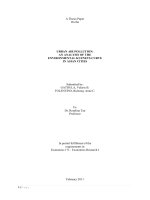
%Figure 2: Relationship between air pollution problems in cities and the level of development. As a
city experiences development, the air pollution problems in the city increase rapidly, before
stabilizing and declining as air pollution controls are implemented (Peters & Murray, 2006)

There are three main economists suggesting the relationship between income and the
environment as well as the reasons for the inverted-U shape of the model: Grossman (1995),
Borghesi (1999) and (Yandle et al., 2004).
Grossman (1995) offers three main explanations as to how exactly income affects the
environment. First, is the ‘scale effect of income on the ‘environment’. As more outputs are
produced, more inputs (natural resources included) are required and more wastes and
emissions as by-products are created during the process. Thus, resulting in the use of more
natural resources to provide inputs and at the same time more polluting by-products leading
to the degradation of the environment. Second, is the technology composition effect. This

refers to the technology as a percent of GDP. A higher technology composition effect
improves the state of the environment as there are more efficient means of manufacturing and
producing goods. A higher technology composition is assumed to imply more sophisticated
end efficient technology that is beneficial for the environment. Last, is the technique effect.
Technique pertains to the research and development (R&D) of a country. Countries with
better techniques experience improving environment conditions as R&D enables the country
to discover means and ways of doing things that are more efficient. That is, technique leads
to the substitution of crude production processes to more efficient and cleaner ones. The first
9"|"P age"
%
effect demonstrates the negative effect of development on the environment, happening during
the early stages. On the other hand, the last two shows how the environment would improve
as brought about by more economic progress.
Furthermore, Borghesi (1999) suggested that market signals or the ‘existence of an
endogenous self-regulatory market mechanism for the use of natural resources’ may also
explain the shape of the EKC. According to him, during the early stages of development there
is heavy exploitation of natural resources leading to a reduction of natural capital. However,
at a certain time, there comes an increase in the price of natural resources. This leads to a
reduction in its exploitation. Furthermore, there is an ‘accelerated shift towards less resource-
intensive technologies’.
In addition, (Yandle et al., 2004) offers another reason as to why the EKC is shaped,
as it is. According to his reasoning, environment quality is a luxury good at higher levels of
income. This indicates that ‘the income elasticity of demand for environmental resources
varies with the level of income’. As a country is at its early stages of development, the
income elasticity for such is less than one. However, after a certain threshold the income
elasticity becomes greater than one. That is, the change in demand for high quality
environment becomes larger than the change in income. The increasing demand for good
quality environment results in an improvement in the environment.
Regarding the limitations of the EKC, Stern (2004) offers a comprehensive study
regarding of its theoretical confines. First, there is ‘no feedback from environmental damage

to economic production given that income is given as an exogenous variable”. It is
immediately assumed that any economic activity done by the country is sustained by the
environment. This might seem problematic because environmental damage might reduce
economic activity; thus, potentially stopping economic growth and development. ‘If higher
levels of economic activity are not sustainable, attempting to grow fast during the early stages
10"|"P age"
%
of development, when environmental degradation is rising, may prove to be
counterproductive’. Second, the decrease in some air pollutant levels as brought about by
greater investment in technology might only mean a shift in the kind of air pollutant now
being produced. In other words, although specific air pollutant levels might be decreasing,
the aggregate might still be the same or even worse.
Third, the effects of trade are not considered in the theory. According to the
Hecksher-Ohlin trade theory, under free trade countries would tend to specialize on economic
activities that the country has abundant resource on. Thus, developed countries would
concentrate on labor and service production while developing countries would put emphasis
on human capital and manufactured capital-intensive activities. As such, this might explain
for the further degradation of environment of the latter, while improvement for the former.
Lastly, stringent environmental policies of the developed countries might lead to
polluting activities gravitating towards developing countries. As a result, ‘these effects would
exaggerate any apparent decline in pollution intensity with rising income along the EKC’.








11"|"P age"

%
B. Empirical
In an empirical analyses of the EKC, two topics are of main interest: first, the
calculation of the threshold where environmental quality improves with rising per capita
income and second, whether a given indicator of environmental degradation displays an
inverted- U relationship in association with rising levels of per capita income.
In terms of the calculated threshold, studies done by Grossman and Krueger (1991),
Shafik and Bandopadhyay (1992) and Selden and Song (1994) would be used as basis of
comparison due to their extensive research and well documented study.
Grossman and Krueger (1991) analyzed the EKC relationship in the context of the
North American Free Trade Agreement (NAFTA) and used the EKC-based hypothesis to
argue that a NAFTA-based trade expansion would protect the environment. They used sulfur
dioxide and dark matter (smoke) suspended in the air in order to estimate the environmental
conditions. Their results showed that turning point came when per capita GDP was in the
range of $4,000 to $5,000 measured in 1985 U.S. dollars, which is approximately $6,700 to
$8,450 in 2003 dollars. Unlike the relationship found for sulfur dioxide and smoke, no
turning point was found for suspended particulates. In this case, the relationship between
pollution and GDP was monotonically increasing. As GDP per capita rose, so did this form of
pollution. (Yandle et al., 2004). Furthermore, Grossman and Krueger’s study looked into the
effect of other factors such as population density and the type of land on pollution levels. As
these factors are not correlated to income level, they are not necessary to make the equation
unbiased. However, Grossman and Krueger noted that the addition of these variables “reduce
residual variance and make the coefficients more precise.” Lastly, the Grossman and Krueger
included the “cubic of average GDP per capita in the preceding three years to proxy for the
effect of permanent income, and because past income is likely to be a relevant determinant of
current environmental standards” (Grossman and Kruegar, 1995). That is, income three years
12"|"P age"
%
before the time period analyzed has an effect on the time period’s pollution levels as
machinery, equipment and activities employed at the current time is a product of income in

the recent past. GDP per capita and the average GDP per capita for the preceding three years
were cubed to allow for greater flexibility in defining the relationship between income and
pollution levels.
Shortly after Grossman and Krueger, Shafik and Bandopadhyay (1992) released their
study done on EKC. They estimated the relationship between economic growth and several
key indicators of environmental quality reported in the World Bank’s cross-country time-
series data sets. They found a consistently significant relationship between income and all
indicators of environmental quality they examined. As income increases from low levels,
quantities of sulfur dioxide, suspended particulate matter, and fecal coliform increase initially
and then decrease once the economy reaches a certain level of income. The turning-point
incomes in 1985 U.S. dollars for these pollutants are $3,700, $3,300 and $1,400
respectively.9 (In 2003 U. S. dollars, the turning points would be about $6,200, $5,500 and
$2,300.) (Yandle et al., 2004)
After two years, Selden and Song (1994) examined the two air pollutants studied by
Grossman and Krueger, along with oxides of nitrogen and carbon monoxide. Their results
lend support to the existence of an EKC relationship for all four air pollutants (sulfur dioxide,
dark matter, nitrogen oxides and carbon monoxide). The EKC turning point (in 1985 U.S.
dollars) for sulfur dioxide was nearly $9,000, and in the vicinity of $10,000 for suspended
particulate matter. (In 2003 dollars, the figures would be about $15,200 and $16,900.) Both
the figures are significantly higher than the estimates from Grossman and Krueger. Seldon
and Song attribute the higher turning points to the use of aggregate air-quality data, which
includes readings from both rural and urban areas, rather than the urban data used by
Grossman and Krueger. The turning-point for environmental pollution was discovered to be
13"|"P age"
%
over $10,000 for oxides of nitrogen, while carbon monoxide peaked when income levels
were a little over $15,000 (or approximately $16,900 and $25,300 in 2003 U.S. dollars)
(Yandle et al., 2004)
In summary, a long series of studies have investigated the relationship between
income and pollution as defined by the Environmental Kutznets Curve. Papers by Grossman

and Krueger (1991), Shafik and Bandyopadhyay (1992) and Selden and Song (1994)
presented evidence that some pollutants have historically followed an inverted U-curve with
respect to income. Although these and other empirical studies point to a correlation between
income and pollution, the causal relation is not observed for all sets of data. That is, there
seems to be a highly specific and controlled environment under which the EKC condition can
be observed. As such, some research like those done by Harbaugh, Levinson and Wilson
(2002), Carson (2009), etc. do not agree with the EKC model due to the limitations of the
theory and the assumptions incorporated in it.
In terms of the shape of the EKC, debates and further studies have shown other
variations from the inverted-U shape originally proposed: cubic function and L-shaped curves.
Torras and Boyce (1998) suggested that instead of a quadratic function, the EKC
actually follows a cubic one. This allows for the possibility that a downturn in pollution (at
the peak of the inverted U) can be followed by a later upturn, that is, a reversal of the
tendency for pollution levels to decline with further increases in per capita income. These
findings imply that beyond some point, high-income levels, rather than being conducive to
further improvement in air and water quality, can have the opposite effect. One possibility is
that the scale effect overshadows the composition and technology effects.



14"|"P age"
%




Figure 3: Environmental Kutznets Cruve: Cubic Function (Torras and Boyce 1998)
Furthermore, a study done by Lucinda Peters and Frank Murray (2006) revealed an L-
shaped EKC as compared to the traditional inverted-U when applied to the Asian context. Air
quality and Gross National Income (GNI) per capita data were collected to create simple

EKC graphs for Asian cities and the air pollutants of SO2, NO2, CO, PM-10 and TSP. The
“L-shape” could be indicative of the traditional EKC inverted U curve, with the original “pre-
pollution” stage no longer applicable in most Asian countries. (Peters & Murray, 2006)
Results show that for Asian countries, Sulphur Dioxide decreased at $520 (US) GNI
per capita; Nitrogen Dioxide on the other hand has either no obvious EKC emerging from the
data. Carbon Monoxide, Particulate Matter (PM10) and Total Suspended Particulates
decreased at approximately $500 (US) GNI per capita (Peters & Murray, 2006)
The study may indicate that for urban air pollution in Asian cities, the typical EKC
shape may not be applicable. The data suggest a lowering of the income turning points for
selected pollutants indicating that at low economic development, Asian cities are
implementing effective air pollution control measures. Instead of the inverted U curve
synonymous with the typical EKC curve, the graphs indicate the emergence of an “L-shape”
EKC for air pollutants in Asian cities. It is proposed that this is due to lowering of income
turning points and the shortening of the stages of economic development accompanying
deteriorating air quality. Furthermore, it is a possible that the “L-shape” EKC is due to the
low number of countries in Asia experiencing the earliest stages of economic development
15"|"P age"
%
and consequential high levels of urban air pollution. This could result in the majority of
countries being near the EKC turning points or in the descending curve, creating the
appearance of an “L-shape” (Peters & Murray, 2006)
Figure 4: Traditional representation of environmental quality Kuznets inverted U curve (red)
versus envisioned EKC (“L-shape”) for selected air pollutants for Asian cities in a modern
environment regulation context (blue). (Peters & Murray, 2006)

16"|"P age"
%
C. Contribution of Paper to the Study of Economics
This research paper, given the recent data of the different air pollutants (PM-10, SO
2

and NO
2
) in several cities in Asia, will utilize the Environmental Kutznets Curve in order to
determine a two-fold goal: first, if the EKC model exists in the Asian context and second, the
GNI per capita that each pollutant would start to decline if ever it does exist. As compared to
the study published by Lucinda Peters and Frank Murray in 2006, this paper is grounded on
scientific data obtained from the Clean Air Initiative- Asia. That is, it will be able to establish
an econometric relationship between income and environment levels for Asian countries.
Furthermore, it would elaborate on possible explanations based on the existence or non-
existence of the EKC. It will more specifically define the relationship between income and
pollution, as well as the impact of Research and Development (R&D) Expenditure, Road
Energy consumption, Capital Formation, and Population Density on pollution levels. The
highly specific relationship that would be obtained could greatly help in the formulation of
timely and essential policies to improve the state of the environment.

17"|"P age"
%
III. THEORETICAL FRAMEWORK
The Environmental Kuznets Curve states that at the early stages of development as
depicted by low levels of per capita income, one can expect rising pollution levels. The rapid
depletion of the environment at low income levels is a result of the increasing use and
depletion of natural resources, rise in emission of pollutants, the operation of less efficient
and relatively dirty technologies, the high priority given to material output, combined with
the low priority and even disregard of the environmental consequences of growth. However,
as economic growth continues and income per capita increases, the EKC projects a slowdown
in environmental pollution and depletion. That is, after a certain income is achieved,
pollution decreases, resulting in the inverse-U shaped curve. As such the EKC is described by
the equation:
Ln(Pollutant) = a + b ln(G
it
)+ c[ln(G
it
))^2]+ u
Pollutants can be any air, water or soil particles that are considered detrimental to

the environment. For this study, 3 of the most widely monitored pollutants are used: PM10,
SO2 and NO2. Taking the logarithm of the pollutant results in a slightly different
interpretation of results the coefficient would be indicative of the effect of the change in the
independent variable on the change in the pollutant. A positive coefficient means that an
increase in the rate of change of per capita GDP results in a similar increase in the rate of
change of pollutant levels. This is different from the interpretation for level variables where a
positive coefficient implies that an increase in the independent variable results in an increase
in the dependent variable. The squaring of the GDP per capita will allow for the
determination of an inverse-U shape as it will reveal the decreasing effect of high levels of
per capita GDP on pollution levels. After all, at high income per capita levels (GDP per
capita) the negative sign of the coefficient of GDP per capita squared will have a decreasing
effect on pollutant levels resulting in the downward turn of the U-shaped curve.
18"|"P age"
%
For this study, the Grossman and Krueger variation of the EKC equation was used
to incorporate more factors that could affect income. A more in depth discussion will be
conducted in the methodology section.

19"|"P age"
%
IV. METHODOLOGY
A. Regression Model
One of the most prominent econometric models formulated to quantify the
Environmental Kuznets Curve (EKC) is that of Grossman and Krueger’s (1995). The
theoretical model states that at the low levels of per capita income, where development and
industrialization is intensive, one can expect rising pollution levels. The rapid depletion of the
environment at low income levels is a result of the increasing use and depletion of natural
resources, rise in emission of pollutants, the operation of less efficient and relatively dirty
technologies, the high priority given to material output, combined with the low priority and
even disregard of the environmental consequences of growth. However, as economic growth
continues and income increases, the EKC projects a slowdown in environmental pollution
and depletion. That is, after a certain income is achieved, pollution decreases, resulting in the
inverse-U curve.
Grossman and Krueger defines the Environmental Kuznets Curve as:


Source: Grossman and Krueger (1991), Economic Growth and the Environment.

The EKC is said to exist if β
1
has a positive sign and

β
2
has a negative sign, resulting

in the inverse-U shaped curve. The Cubic part is there only to provide for a more accurate
measure of the relationship. If indeed there is a U-shaped curve, β
3
will have the same
negative sign as β
2,
implying it will continue to decrease pollution levels. Or alternatively, an
insignificant β
3
also shows that the square is a sufficient indicator of the income-pollution
relationship.
20"|"P age"
%
In addition to the population density factor looked into by Grossman and Krueger,
this paper added 3 other variables: Industry value (% of GDP from industrial sector), Road
Sector Energy Consumption, and Gross Capital Formation. R&D Expenditure pertains to the
amount of money invested in R&D in relation to the country’s total GDP. The World Bank
defines Road Sector Energy consumption as the “total energy used in the road sector
including petroleum products, natural gas, electricity, and combustible renewable waste.”
This is indicative of the level of vehicle activity which inevitable affects pollution levels. Last,
this paper also looks into gross capital formation or the “outlays on additions to the fixed
assets of the economy plus net changes in the level of inventories.” (World Bank) The level
of capital formation is indicative of industrial and economic activity including “land
improvements (fences, ditches, drains, and so on); plant, machinery, and equipment
purchases; and the construction of roads, railways, and the like, including schools, offices,
hospitals, private residential dwellings, and commercial and industrial buildings. Inventories
are stocks of goods held by firms to meet temporary or unexpected fluctuations in production
or sales.” That is, higher capital formation is indicative of higher industrial and economic
construction resulting in pollution a few years hence.

The equations used for this study are as follows:
PM-10 = a + b G
it
+ c G
it
^2+ d G
it
^3+ e G
it
+ f G
it
^2+ g G
it
^3 + X
it
+ u
PM-10= a + b G
it
+ c G
it
^2+ + d G
it
+ e G
it
^2+ + X
it
+ u
SO
2
= a + b G

it
+ c G
it
^2+ d G
it
^3+ e G
it
+ f G
it
^2+ g G
it
^3 + X
it
+ u
SO
2
= a + b G
it
+ c G
it
^2+ + d G
it
+ e G
it
^2+ X
it
+ u
NO
2
= a + b G

it
+ c G
it
^2+ + d G
it
+ e G
it
^2+ X
it
+ u
NO
2
= a + b G
it
+ c G
it
^2+ + d G
it
+ e G
it
^2+ X
it
+u
21"|"P age"
%

The dependent or endogenous variable is the pollutant level, PM10, SO2 and NO2,
while the independent or exogenous variables are the Gross Domestic Product (GDP) per
capita as represented by Git, the square of Git, the cube of Git, Git or the 3 year GDP per
capita lag variable (computed as the average of GDP per capita 3 years before time t), Git^2,

Git^3 and Xit. Grossman and Kruegar used Xit as a representation for population density,
land use, and distance from desert areas. For this study, Xit stands for population density,
industrial level, Road Sector Energy Consumption and Gross Capita Formation.
Environmental condition is depicted by the level of air pollutant while development is
captured by the income per capita. The square measures nonlinearities in the time path of
pollution while the cube allows for flexibility in determining the relationship between income
and pollution. An EKC relationship will result in an insignificant coefficient for the cubic
factors, as well as a positive sign for income per capita and lagged income per capita, and a
negative sign for their respective squares. Thus, supporting the inversed U-shape of the
theory.
The potential source for the fragility of the results can be brought about by multi-
collinearity. As might be expected, there is a high degree of correlation between the per
capita income, its square, cube and lagged versions.


22"|"P age"
%
B. Data


For the Yit or the pollutant level, Particulate Matter (PM-10), Sulfur Dioxide (SO
2
)
and Nitrogen Dioxide (NO
2
) levels would be utilized. The data was gathered from Clean Air
Initiative- Asia (CAI-Asia, 2010).
According to literature, among air pollutants, these three are the more documented
ones as these are some of the ones earlier discovered leading to the development of capacity
to measure such compounds. Also, it is important to consider the three pollutants due to their

pressing effects on health and their impact on society. First, PM10 is a major pollutant in
Asian cities—with the average of annual average PM10 concentrations over three times
above the WHO guidelines since 1993 (CAI-Asia, 2010). PM-10 is produced through natural
activities (e.g. Volcanic eruptions, fire, living vegetation, etc.) and man-made (e.g. use of
fossil fuels and other industrial activities). It is made up of a number of components,
including acids, organic chemicals, metals, and soil or dust particles. The size of particles is
inversely proportional to their potential for causing health problems. That is, smaller particles
are more harmful as it is more difficult for these to be removed from the body system. These
particles stay longer in the body and cause more harm. The United States Environmental
Protection Agency (US EPA) is concerned about particles that are 10 micrometers in
diameter or smaller because those are the particles that generally easily through the throat and
nose and enter the lungs. Once inhaled, these particles can affect the heart and lungs and
cause serious health effects (2010). The largest sources of SO
2
emissions are from fossil fuel
combustion at power plants and other industrial facilities. Smaller sources of SO
2
emissions
23"|"P age"
%
include industrial processes such as extracting metal from ore, and the burning of high sulfur
containing fuels by locomotives, large ships, and non-road equipment. Exposure to this
pollutant causes an array of adverse respiratory effects including bronchoconstriction and
increased asthma symptoms (US EPA, 2010). Third, NO
2
forms quickly from emissions from
cars, trucks and buses, power plants, and off-road equipment. In addition to contributing to
the formation of ground-level ozone, and fine particle pollution, NO
2
is linked with a number

of adverse effects on the respiratory system (US EPA, 2010).
The Gross Domestic Product was calculated at purchaser's prices is the sum of gross
value added by all resident producers in the economy plus any product taxes and minus any
subsidies not included in the value of the products. It is calculated without making deductions
for depreciation of fabricated assets or for depletion and degradation of natural resources.
Data are in current U.S. dollars. Dollar figures for GDP are converted from domestic
currencies using single year official exchange rates. For a few countries where the official
exchange rate does not reflect the rate effectively applied to actual foreign exchange
transactions, an alternative conversion factor is used. The data was sourced from World Bank
national accounts data, and OECD National Accounts data files. Using this data, the lagged
variables were easy to determine (World Bank, 2011).
Industry value, Road Sector Energy consumption and Gross Capital Formation data
were all obtained from the World bank database.
The seven countries observed for PM-10 and SO
2
are: China, Hong Kong, India,
Japan, Korea, Singapore, and Thailand. For NO
2
, the five countries observed are: Hong Kong,
India, Japan, Singapore and Thailand. While the NO2 regression involved: Hong Kong,
Japan and Singapore. For all regressions, data for years 1998-2005 were used. The timeframe
of the paper’s analysis is only for eight years due to the constraints in pollutant level data.
24"|"P age"
%
Furthermore, the capital of the country was chosen to represent that nation’s status of air
quality as this city contains the most data.
Regression for panel data was conducted, controlling for time differences through the
fixed effects model. That is, the data points were taken as non-random occurrences, and the
model controlled for factors in such a way that characteristics of the data do not change over
time.

C. Results
Square Regression for all Countries (China, Hong Kong, India, Japan, Korea, Singapore and
Thailand; 1998-2005)


Dependent Variable


Ln_PM10
Ln_SO2
Ln_NO2
Constant
163.209
155.023*
-83.1702
GDP
0.000987631
-0.00102903
0.00515503
GDP_sq
1.93925e-08
2.48542e-08
-8.65557e-08
Lagged_GDP
-0.0111811*
-0.00480846
0.00376252
Lagged_GDP_2
2.36770e-07**
1.22719e-07

-8.14665e-08
Population Density
-0.00123877
-0.00843698
-0.0102944
Road Sector
Energy
Consumption
-1.62134**
-1.72679**
0.354297
Gross Capital
Formation (-9)
-1.93209**
-0.495216
0.0049***
R-squared
0.975041
0.909464
0.951947
Adjusted R-
squared
0.958402
0.849107
0.906297

Given that β
3
exponents were not significant, these were no longer taken into
consideration. The summarized results of regression with cubic parameters can be seen in the

Appendix section.
25"|"P age"
%
The negative sign of Lagged_GDP for PM-10 (the only case where the variable was
significant) is interpreted as: an increase in the average GDP per capita in the 3 preceding
years will result in a decrease in pollution levels. However, at high income levels, the
positive sign of Lagged_GDP_2 for PM-10 is interpreted as resulting in an increase in
pollution levels in the long-run. This results in a U-shaped curve, instead of the inverse-U
defined by the EKC. This may be explained by the fact that the low-income countries (China,
India and Thailand) are not primarily agricultural economies with low level of pollution. On
the contrary, China, India and Thailand actually have industrial activities of a similar
magnitude to developed countries such as Hong Kong, Japan, Singapore and Korea. That is,
the low income countries are not agricultural economies expected to emit low level of
pollutants. The EKC phenomenon assumes that there is a low level of pollution at low
income levels because the low income level is a result of an agricultural economy which
emits less pollutant. However, this clearly does not hold for the data points where there is a
low income level. At the low income level data points, there are high pollution levels as well
as high industry activity, high energy consumption and capital formation.
The negative sign of the coefficient of the Road Sector Energy consumption variable
for PM-10 and SO2 data indicates that an increase in energy consumption results in a
decrease in pollution levels. This is quite counterintuitive as more energy consumption
usually results in an increase in pollution level because of by-products of the activity.
However, more efficient car technology may explain for this phenomenon. More efficient car
technology (which is becoming the norm in high income countries) harness other sources of
energy (electricity, water, etc.) leading to a decrease in pollution levels amidst rising energy
consumption. Evidence of this can be seen in the increase in hybrid cars, more energy
efficient, etc.