Learning Deep Architectures for AI Yoshua Bengio Dept IRO

1

Learning Deep Architectures for AI
Yoshua Bengio
Dept. IRO, Universit´e de Montr´eal
C.P. 6128, Montreal, Qc, H3C 3J7, Canada

/>To appear in Foundations and Trends in Machine Learning
Abstract
Theoretical results suggest that in order to learn the kind of complicated functions that can represent highlevel abstractions (e.g. in vision, language, and other AI-level tasks), one may need deep architectures.
Deep architectures are composed of multiple levels of non-linear operations, such as in neural nets with
many hidden layers or in complicated propositional formulae re-using many sub-formulae. Searching the
parameter space of deep architectures is a difficult task, but learning algorithms such as those for Deep
Belief Networks have recently been proposed to tackle this problem with notable success, beating the
state-of-the-art in certain areas. This paper discusses the motivations and principles regarding learning
algorithms for deep architectures, in particular those exploiting as building blocks unsupervised learning
of single-layer models such as Restricted Boltzmann Machines, used to construct deeper models such as
Deep Belief Networks.

1

Introduction

Allowing computers to model our world well enough to exhibit what we call intelligence has been the focus
of more than half a century of research. To achieve this, it is clear that a large quantity of information
about our world should somehow be stored, explicitly or implicitly, in the computer. Because it seems
daunting to formalize manually all that information in a form that computers can use to answer questions
and generalize to new contexts, many researchers have turned to learning algorithms to capture a large
fraction of that information. Much progress has been made to understand and improve learning algorithms,
but the challenge of artificial intelligence (AI) remains. Do we have algorithms that can understand scenes
and describe them in natural language? Not really, except in very limited settings. Do we have algorithms

that can infer enough semantic concepts to be able to interact with most humans using these concepts? No.
If we consider image understanding, one of the best specified of the AI tasks, we realize that we do not yet
have learning algorithms that can discover the many visual and semantic concepts that would seem to be
necessary to interpret most images on the web. The situation is similar for other AI tasks.
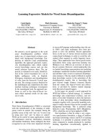
Consider for example the task of interpreting an input image such as the one in Figure 1. When humans
try to solve a particular AI task (such as machine vision or natural language processing), they often exploit
their intuition about how to decompose the problem into sub-problems and multiple levels of representation,
e.g., in object parts and constellation models (Weber, Welling, & Perona, 2000; Niebles & Fei-Fei, 2007;
Sudderth, Torralba, Freeman, & Willsky, 2007) where models for parts can be re-used in different object instances. For example, the current state-of-the-art in machine vision involves a sequence of modules starting
from pixels and ending in a linear or kernel classifier (Pinto, DiCarlo, & Cox, 2008; Mutch & Lowe, 2008),
with intermediate modules mixing engineered transformations and learning, e.g. first extracting low-level


features that are invariant to small geometric variations (such as edge detectors from Gabor filters), transforming them gradually (e.g. to make them invariant to contrast changes and contrast inversion, sometimes
by pooling and sub-sampling), and then detecting the most frequent patterns. A plausible and common way
to extract useful information from a natural image involves transforming the raw pixel representation into
gradually more abstract representations, e.g., starting from the presence of edges, the detection of more complex but local shapes, up to the identification of abstract categories associated with sub-objects and objects
which are parts of the image, and putting all these together to capture enough understanding of the scene to
answer questions about it.
Here, we assume that the computational machinery necessary to express complex behaviors (which one
might label “intelligent”) requires highly varying mathematical functions, i.e. mathematical functions that
are highly non-linear in terms of raw sensory inputs, and display a very large number of variations (ups and
downs) across the domain of interest. We view the raw input to the learning system as a high dimensional
entity, made of many observed variables, which are related by unknown intricate statistical relationships. For
example, using knowledge of the 3D geometry of solid objects and lighting, we can relate small variations in
underlying physical and geometric factors (such as position, orientation, lighting of an object) with changes
in pixel intensities for all the pixels in an image. We call these factors of variation because they are different
aspects of the data that can vary separately and often independently. In this case, explicit knowledge of
the physical factors involved allows one to get a picture of the mathematical form of these dependencies,
and of the shape of the set of images (as points in a high-dimensional space of pixel intensities) associated

with the same 3D object. If a machine captured the factors that explain the statistical variations in the data,
and how they interact to generate the kind of data we observe, we would be able to say that the machine
understands those aspects of the world covered by these factors of variation. Unfortunately, in general and
for most factors of variation underlying natural images, we do not have an analytical understanding of these
factors of variation. We do not have enough formalized prior knowledge about the world to explain the
observed variety of images, even for such an apparently simple abstraction as MAN, illustrated in Figure 1.
A high-level abstraction such as MAN has the property that it corresponds to a very large set of possible
images, which might be very different from each other from the point of view of simple Euclidean distance
in the space of pixel intensities. The set of images for which that label could be appropriate forms a highly
convoluted region in pixel space that is not even necessarily a connected region. The MAN category can be
seen as a high-level abstraction with respect to the space of images. What we call abstraction here can be a
category (such as the MAN category) or a feature, a function of sensory data, which can be discrete (e.g., the
input sentence is at the past tense) or continuous (e.g., the input video shows an object moving at
2 meter/second). Many lower-level and intermediate-level concepts (which we also call abstractions here)
would be useful to construct a MAN-detector. Lower level abstractions are more directly tied to particular
percepts, whereas higher level ones are what we call “more abstract” because their connection to actual
percepts is more remote, and through other, intermediate-level abstractions.
In addition to the difficulty of coming up with the appropriate intermediate abstractions, the number of
visual and semantic categories (such as MAN) that we would like an “intelligent” machine to capture is
rather large. The focus of deep architecture learning is to automatically discover such abstractions, from the
lowest level features to the highest level concepts. Ideally, we would like learning algorithms that enable
this discovery with as little human effort as possible, i.e., without having to manually define all necessary
abstractions or having to provide a huge set of relevant hand-labeled examples. If these algorithms could
tap into the huge resource of text and images on the web, it would certainly help to transfer much of human
knowledge into machine-interpretable form.

1.1

How do We Train Deep Architectures?

Deep learning methods aim at learning feature hierarchies with features from higher levels of the hierarchy
formed by the composition of lower level features. Automatically learning features at multiple levels of
abstraction allows a system to learn complex functions mapping the input to the output directly from data,

2


Figure 1: We would like the raw input image to be transformed into gradually higher levels of representation,
representing more and more abstract functions of the raw input, e.g., edges, local shapes, object parts,
etc. In practice, we do not know in advance what the “right” representation should be for all these levels
of abstractions, although linguistic concepts might help guessing what the higher levels should implicitly
represent.

3


without depending completely on human-crafted features. This is especially important for higher-level abstractions, which humans often do not know how to specify explicitly in terms of raw sensory input. The
ability to automatically learn powerful features will become increasingly important as the amount of data
and range of applications to machine learning methods continues to grow.
Depth of architecture refers to the number of levels of composition of non-linear operations in the function learned. Whereas most current learning algorithms correspond to shallow architectures (1, 2 or 3 levels),
the mammal brain is organized in a deep architecture (Serre, Kreiman, Kouh, Cadieu, Knoblich, & Poggio,
2007) with a given input percept represented at multiple levels of abstraction, each level corresponding to
a different area of cortex. Humans often describe such concepts in hierarchical ways, with multiple levels
of abstraction. The brain also appears to process information through multiple stages of transformation and
representation. This is particularly clear in the primate visual system (Serre et al., 2007), with its sequence
of processing stages: detection of edges, primitive shapes, and moving up to gradually more complex visual
shapes.
Inspired by the architectural depth of the brain, neural network researchers had wanted for decades to
train deep multi-layer neural networks (Utgoff & Stracuzzi, 2002; Bengio & LeCun, 2007), but no successful attempts were reported before 20061: researchers reported positive experimental results with typically
two or three levels (i.e. one or two hidden layers), but training deeper networks consistently yielded poorer

results. Something that can be considered a breakthrough happened in 2006: Hinton and collaborators at
U. of Toronto introduced Deep Belief Networks or DBNs for short (Hinton, Osindero, & Teh, 2006), with
a learning algorithm that greedily trains one layer at a time, exploiting an unsupervised learning algorithm
for each layer, a Restricted Boltzmann Machine (RBM) (Freund & Haussler, 1994). Shortly after, related
algorithms based on auto-encoders were proposed (Bengio, Lamblin, Popovici, & Larochelle, 2007; Ranzato, Poultney, Chopra, & LeCun, 2007), apparently exploiting the same principle: guiding the training of
intermediate levels of representation using unsupervised learning, which can be performed locally at each
level. Other algorithms for deep architectures were proposed more recently that exploit neither RBMs nor
auto-encoders and that exploit the same principle (Weston, Ratle, & Collobert, 2008; Mobahi, Collobert, &
Weston, 2009) (see Section 4).
Since 2006, deep networks have been applied with success not only in classification tasks (Bengio et al.,
2007; Ranzato et al., 2007; Larochelle, Erhan, Courville, Bergstra, & Bengio, 2007; Ranzato, Boureau, &
LeCun, 2008; Vincent, Larochelle, Bengio, & Manzagol, 2008; Ahmed, Yu, Xu, Gong, & Xing, 2008; Lee,
Grosse, Ranganath, & Ng, 2009), but also in regression (Salakhutdinov & Hinton, 2008), dimensionality reduction (Hinton & Salakhutdinov, 2006a; Salakhutdinov & Hinton, 2007a), modeling textures (Osindero &
Hinton, 2008), modeling motion (Taylor, Hinton, & Roweis, 2007; Taylor & Hinton, 2009), object segmentation (Levner, 2008), information retrieval (Salakhutdinov & Hinton, 2007b; Ranzato & Szummer, 2008;
Torralba, Fergus, & Weiss, 2008), robotics (Hadsell, Erkan, Sermanet, Scoffier, Muller, & LeCun, 2008),
natural language processing (Collobert & Weston, 2008; Weston et al., 2008; Mnih & Hinton, 2009), and
collaborative filtering (Salakhutdinov, Mnih, & Hinton, 2007). Although auto-encoders, RBMs and DBNs
can be trained with unlabeled data, in many of the above applications, they have been successfully used to
initialize deep supervised feedforward neural networks applied to a specific task.

1.2

Intermediate Representations: Sharing Features and Abstractions Across Tasks

Since a deep architecture can be seen as the composition of a series of processing stages, the immediate
question that deep architectures raise is: what kind of representation of the data should be found as the output of each stage (i.e., the input of another)? What kind of interface should there be between these stages? A
hallmark of recent research on deep architectures is the focus on these intermediate representations: the success of deep architectures belongs to the representations learned in an unsupervised way by RBMs (Hinton
et al., 2006), ordinary auto-encoders (Bengio et al., 2007), sparse auto-encoders (Ranzato et al., 2007, 2008),
or denoising auto-encoders (Vincent et al., 2008). These algorithms (described in more detail in Section 7.2)
1 Except

for neural networks with a special structure called convolutional networks, discussed in Section 4.5.

4


can be seen as learning to transform one representation (the output of the previous stage) into another, at
each step maybe disentangling better the factors of variations underlying the data. As we discuss at length
in Section 4, it has been observed again and again that once a good representation has been found at each
level, it can be used to initialize and successfully train a deep neural network by supervised gradient-based
optimization.
Each level of abstraction found in the brain consists of the “activation” (neural excitation) of a small
subset of a large number of features that are, in general, not mutually exclusive. Because these features
are not mutually exclusive, they form what is called a distributed representation (Hinton, 1986; Rumelhart,
Hinton, & Williams, 1986b): the information is not localized in a particular neuron but distributed across
many. In addition to being distributed, it appears that the brain uses a representation that is sparse: only
around 1-4% of the neurons are active together at a given time (Attwell & Laughlin, 2001; Lennie, 2003).
Section 3.2 introduces the notion of sparse distributed representation and 7.1 describes in more detail the
machine learning approaches, some inspired by the observations of the sparse representations in the brain,
that have been used to build deep architectures with sparse representations.
Whereas dense distributed representations are one extreme of a spectrum, and sparse representations are
in the middle of that spectrum, purely local representations are the other extreme. Locality of representation
is intimately connected with the notion of local generalization. Many existing machine learning methods are
local in input space: to obtain a learned function that behaves differently in different regions of data-space,
they require different tunable parameters for each of these regions (see more in Section 3.1). Even though
statistical efficiency is not necessarily poor when the number of tunable parameters is large, good generalization can be obtained only when adding some form of prior (e.g. that smaller values of the parameters are
preferred). When that prior is not task-specific, it is often one that forces the solution to be very smooth, as
discussed at the end of Section 3.1. In contrast to learning methods based on local generalization, the total
number of patterns that can be distinguished using a distributed representation scales possibly exponentially
with the dimension of the representation (i.e. the number of learned features).

In many machine vision systems, learning algorithms have been limited to specific parts of such a processing chain. The rest of the design remains labor-intensive, which might limit the scale of such systems.
On the other hand, a hallmark of what we would consider intelligent machines includes a large enough repertoire of concepts. Recognizing MAN is not enough. We need algorithms that can tackle a very large set of
such tasks and concepts. It seems daunting to manually define that many tasks, and learning becomes essential in this context. Furthermore, it would seem foolish not to exploit the underlying commonalities between
these tasks and between the concepts they require. This has been the focus of research on multi-task learning (Caruana, 1993; Baxter, 1995; Intrator & Edelman, 1996; Thrun, 1996; Baxter, 1997). Architectures
with multiple levels naturally provide such sharing and re-use of components: the low-level visual features
(like edge detectors) and intermediate-level visual features (like object parts) that are useful to detect MAN
are also useful for a large group of other visual tasks. Deep learning algorithms are based on learning intermediate representations which can be shared across tasks. Hence they can leverage unsupervised data and
data from similar tasks (Raina, Battle, Lee, Packer, & Ng, 2007) to boost performance on large and challenging problems that routinely suffer from a poverty of labelled data, as has been shown by Collobert and
Weston (2008), beating the state-of-the-art in several natural language processing tasks. A similar multi-task
approach for deep architectures was applied in vision tasks by Ahmed et al. (2008). Consider a multi-task
setting in which there are different outputs for different tasks, all obtained from a shared pool of high-level
features. The fact that many of these learned features are shared among m tasks provides sharing of statistical strength in proportion to m. Now consider that these learned high-level features can themselves be
represented by combining lower-level intermediate features from a common pool. Again statistical strength
can be gained in a similar way, and this strategy can be exploited for every level of a deep architecture.
In addition, learning about a large set of interrelated concepts might provide a key to the kind of broad
generalizations that humans appear able to do, which we would not expect from separately trained object
detectors, with one detector per visual category. If each high-level category is itself represented through
a particular distributed configuration of abstract features from a common pool, generalization to unseen

5


categories could follow naturally from new configurations of these features. Even though only some configurations of these features would be present in the training examples, if they represent different aspects of the
data, new examples could meaningfully be represented by new configurations of these features.

1.3

Desiderata for Learning AI

Summarizing some of the above issues, and trying to put them in the broader perspective of AI, we put

forward a number of requirements we believe to be important for learning algorithms to approach AI, many
of which motivate the research described here:
• Ability to learn complex, highly-varying functions, i.e., with a number of variations much greater than
the number of training examples.
• Ability to learn with little human input the low-level, intermediate, and high-level abstractions that
would be useful to represent the kind of complex functions needed for AI tasks.
• Ability to learn from a very large set of examples: computation time for training should scale well
with the number of examples, i.e. close to linearly.
• Ability to learn from mostly unlabeled data, i.e. to work in the semi-supervised setting, where not all
the examples come with complete and correct semantic labels.
• Ability to exploit the synergies present across a large number of tasks, i.e. multi-task learning. These
synergies exist because all the AI tasks provide different views on the same underlying reality.
• Strong unsupervised learning (i.e. capturing most of the statistical structure in the observed data),
which seems essential in the limit of a large number of tasks and when future tasks are not known
ahead of time.
Other elements are equally important but are not directly connected to the material in this paper. They
include the ability to learn to represent context of varying length and structure (Pollack, 1990), so as to
allow machines to operate in a context-dependent stream of observations and produce a stream of actions,
the ability to make decisions when actions influence the future observations and future rewards (Sutton &
Barto, 1998), and the ability to influence future observations so as to collect more relevant information about
the world, i.e. a form of active learning (Cohn, Ghahramani, & Jordan, 1995).

1.4

Outline of the Paper

Section 2 reviews theoretical results (which can be skipped without hurting the understanding of the remainder) showing that an architecture with insufficient depth can require many more computational elements,
potentially exponentially more (with respect to input size), than architectures whose depth is matched to the
task. We claim that insufficient depth can be detrimental for learning. Indeed, if a solution to the task is
represented with a very large but shallow architecture (with many computational elements), a lot of training

examples might be needed to tune each of these elements and capture a highly-varying function. Section 3.1
is also meant to motivate the reader, this time to highlight the limitations of local generalization and local
estimation, which we expect to avoid using deep architectures with a distributed representation (Section 3.2).
In later sections, the paper describes and analyzes some of the algorithms that have been proposed to train
deep architectures. Section 4 introduces concepts from the neural networks literature relevant to the task of
training deep architectures. We first consider the previous difficulties in training neural networks with many
layers, and then introduce unsupervised learning algorithms that could be exploited to initialize deep neural
networks. Many of these algorithms (including those for the RBM) are related to the auto-encoder: a simple
unsupervised algorithm for learning a one-layer model that computes a distributed representation for its
input (Rumelhart et al., 1986b; Bourlard & Kamp, 1988; Hinton & Zemel, 1994). To fully understand RBMs
6


and many related unsupervised learning algorithms, Section 5 introduces the class of energy-based models,
including those used to build generative models with hidden variables such as the Boltzmann Machine.
Section 6 focus on the greedy layer-wise training algorithms for Deep Belief Networks (DBNs) (Hinton
et al., 2006) and Stacked Auto-Encoders (Bengio et al., 2007; Ranzato et al., 2007; Vincent et al., 2008).
Section 7 discusses variants of RBMs and auto-encoders that have been recently proposed to extend and
improve them, including the use of sparsity, and the modeling of temporal dependencies. Section 8 discusses
algorithms for jointly training all the layers of a Deep Belief Network using variational bounds. Finally, we
consider in Section 9 forward looking questions such as the hypothesized difficult optimization problem
involved in training deep architectures. In particular, we follow up on the hypothesis that part of the success
of current learning strategies for deep architectures is connected to the optimization of lower layers. We
discuss the principle of continuation methods, which minimize gradually less smooth versions of the desired
cost function, to make a dent in the optimization of deep architectures.

2

Theoretical Advantages of Deep Architectures

In this section, we present a motivating argument for the study of learning algorithms for deep architectures,
by way of theoretical results revealing potential limitations of architectures with insufficient depth. This part
of the paper (this section and the next) motivates the algorithms described in the later sections, and can be
skipped without making the remainder difficult to follow.
The main point of this section is that some functions cannot be efficiently represented (in terms of number
of tunable elements) by architectures that are too shallow. These results suggest that it would be worthwhile
to explore learning algorithms for deep architectures, which might be able to represent some functions
otherwise not efficiently representable. Where simpler and shallower architectures fail to efficiently represent
(and hence to learn) a task of interest, we can hope for learning algorithms that could set the parameters of a
deep architecture for this task.
We say that the expression of a function is compact when it has few computational elements, i.e. few
degrees of freedom that need to be tuned by learning. So for a fixed number of training examples, and short of
other sources of knowledge injected in the learning algorithm, we would expect that compact representations
of the target function2 would yield better generalization.
More precisely, functions that can be compactly represented by a depth k architecture might require an
exponential number of computational elements to be represented by a depth k − 1 architecture. Since the
number of computational elements one can afford depends on the number of training examples available to
tune or select them, the consequences are not just computational but also statistical: poor generalization may
be expected when using an insufficiently deep architecture for representing some functions.
We consider the case of fixed-dimension inputs, where the computation performed by the machine can
be represented by a directed acyclic graph where each node performs a computation that is the application
of a function on its inputs, each of which is the output of another node in the graph or one of the external
inputs to the graph. The whole graph can be viewed as a circuit that computes a function applied to the
external inputs. When the set of functions allowed for the computation nodes is limited to logic gates, such
as { AND, OR, NOT }, this is a Boolean circuit, or logic circuit.
To formalize the notion of depth of architecture, one must introduce the notion of a set of computational
elements. An example of such a set is the set of computations that can be performed logic gates. Another is
the set of computations that can be performed by an artificial neuron (depending on the values of its synaptic
weights). A function can be expressed by the composition of computational elements from a given set. It
is defined by a graph which formalizes this composition, with one node per computational element. Depth

of architecture refers to the depth of that graph, i.e. the longest path from an input node to an output node.
When the set of computational elements is the set of computations an artificial neuron can perform, depth
corresponds to the number of layers in a neural network. Let us explore the notion of depth with examples
2 The

target function is the function that we would like the learner to discover.

7


output

output

*
element
set

element
set

sin

neuron

*

+

neuron

neuron

neuron

sin
+

neuron

...
*

neuron neuron neuron

neuron

−
x

a

b

inputs

inputs

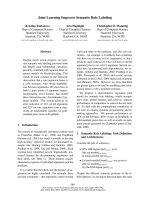
Figure 2: Examples of functions represented by a graph of computations, where each node is taken in some
“element set” of allowed computations. Left: the elements are {∗, +, −, sin}∪R. The architecture computes

x∗sin(a∗x+b) and has depth 4. Right: the elements are artificial neurons computing f (x) = tanh(b+w′ x);
each element in the set has a different (w, b) parameter. The architecture is a multi-layer neural network of
depth 3.
of architectures of different depths. Consider the function f (x) = x ∗ sin(a ∗ x + b). It can be expressed
as the composition of simple operations such as addition, subtraction, multiplication, and the sin operation,
as illustrated in Figure 2. In the example, there would be a different node for the multiplication a ∗ x and
for the final multiplication by x. Each node in the graph is associated with an output value obtained by
applying some function on input values that are the outputs of other nodes of the graph. For example, in a
logic circuit each node can compute a Boolean function taken from a small set of Boolean functions. The
graph as a whole has input nodes and output nodes and computes a function from input to output. The depth
of an architecture is the maximum length of a path from any input of the graph to any output of the graph,
i.e. 4 in the case of x ∗ sin(a ∗ x + b) in Figure 2.
• If we include affine operations and their possible composition with sigmoids in the set of computational elements, linear regression and logistic regression have depth 1, i.e., have a single level.
• When we put a fixed kernel computation K(u, v) in the set of allowed operations, along with affine
operations, kernel machines (Schăolkopf, Burges, & Smola, 1999a) with a fixed kernel can be considered to have two levels. The first level has one element computing K(x, xi ) for each prototype xi (a
selected representative training example) and matches the input vector x with the prototypes xi . The
second level performs an affine combination b + i αi K(x, xi ) to associate the matching prototypes
xi with the expected response.
• When we put artificial neurons (affine transformation followed by a non-linearity) in our set of elements, we obtain ordinary multi-layer neural networks (Rumelhart et al., 1986b). With the most
common choice of one hidden layer, they also have depth two (the hidden layer and the output layer).
• Decision trees can also be seen as having two levels, as discussed in Section 3.1.
• Boosting (Freund & Schapire, 1996) usually adds one level to its base learners: that level computes a
vote or linear combination of the outputs of the base learners.
• Stacking (Wolpert, 1992) is another meta-learning algorithm that adds one level.
• Based on current knowledge of brain anatomy (Serre et al., 2007), it appears that the cortex can be
seen as a deep architecture, with 5 to 10 levels just for the visual system.

8

Although depth depends on the choice of the set of allowed computations for each element, graphs
associated with one set can often be converted to graphs associated with another by an graph transformation
in a way that multiplies depth. Theoretical results suggest that it is not the absolute number of levels that
matters, but the number of levels relative to how many are required to represent efficiently the target function
(with some choice of set of computational elements).

2.1

Computational Complexity

The most formal arguments about the power of deep architectures come from investigations into computational complexity of circuits. The basic conclusion that these results suggest is that when a function can be
compactly represented by a deep architecture, it might need a very large architecture to be represented by
an insufficiently deep one.
A two-layer circuit of logic gates can represent any Boolean function (Mendelson, 1997). Any Boolean
function can be written as a sum of products (disjunctive normal form: AND gates on the first layer with
optional negation of inputs, and OR gate on the second layer) or a product of sums (conjunctive normal
form: OR gates on the first layer with optional negation of inputs, and AND gate on the second layer).
To understand the limitations of shallow architectures, the first result to consider is that with depth-two
logical circuits, most Boolean functions require an exponential (with respect to input size) number of logic
gates (Wegener, 1987) to be represented.
More interestingly, there are functions computable with a polynomial-size logic gates circuit of depth k
that require exponential size when restricted to depth k − 1 (H˚astad, 1986). The proof of this theorem relies
on earlier results (Yao, 1985) showing that d-bit parity circuits of depth 2 have exponential size. The d-bit
parity function is defined as usual:
parity : (b1 , . . . , bd ) ∈ {0, 1}d →

d

1 if
i=1 bi is even

0 otherwise.

One might wonder whether these computational complexity results for Boolean circuits are relevant to
machine learning. See Orponen (1994) for an early survey of theoretical results in computational complexity
relevant to learning algorithms. Interestingly, many of the results for Boolean circuits can be generalized to
architectures whose computational elements are linear threshold units (also known as artificial neurons (McCulloch & Pitts, 1943)), which compute
f (x) = 1w′ x+b≥0

(1)

with parameters w and b. The fan-in of a circuit is the maximum number of inputs of a particular element.
Circuits are often organized in layers, like multi-layer neural networks, where elements in a layer only take
their input from elements in the previous layer(s), and the first layer is the neural network input. The size of
a circuit is the number of its computational elements (excluding input elements, which do not perform any
computation).
Of particular interest is the following theorem, which applies to monotone weighted threshold circuits
(i.e. multi-layer neural networks with linear threshold units and positive weights) when trying to represent a
function compactly representable with a depth k circuit:
Theorem 2.1. A monotone weighted threshold circuit of depth k − 1 computing a function fk ∈ Fk,N has
size at least 2cN for some constant c > 0 and N > N0 (H˚astad & Goldmann, 1991).
The class of functions Fk,N is defined as follows. It contains functions with N 2k−2 inputs, defined by a
depth k circuit that is a tree. At the leaves of the tree there are unnegated input variables, and the function
value is at the root. The i-th level from the bottom consists of AND gates when i is even and OR gates when
i is odd. The fan-in at the top and bottom level is N and at all other levels it is N 2 .
The above results do not prove that other classes of functions (such as those we want to learn to perform
AI tasks) require deep architectures, nor that these demonstrated limitations apply to other types of circuits.
9


However, these theoretical results beg the question: are the depth 1, 2 and 3 architectures (typically found

in most machine learning algorithms) too shallow to represent efficiently more complicated functions of the
kind needed for AI tasks? Results such as the above theorem also suggest that there might be no universally
right depth: each function (i.e. each task) might require a particular minimum depth (for a given set of
computational elements). We should therefore strive to develop learning algorithms that use the data to
determine the depth of the final architecture. Note also that recursive computation defines a computation
graph whose depth increases linearly with the number of iterations.

(x1x2)(x2x3) + (x1x2)(x3x4) + (x2 x3)2 + (x2x3)(x3x4)
×

(x1x2) + (x2x3)
+

x2x3

x1 x2
×

x1

(x2x3 ) + (x3x4)
+

x3 x4
×

×

x2

x3

x4

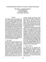
Figure 3: Example of polynomial circuit (with products on odd layers and sums on even ones) illustrating
the factorization enjoyed by a deep architecture. For example the level-1 product x2 x3 would occur many
times (exponential in depth) in a depth 2 (sum of product) expansion of the above polynomial.

2.2

Informal Arguments

Depth of architecture is connected to the notion of highly-varying functions. We argue that, in general, deep
architectures can compactly represent highly-varying functions which would otherwise require a very large
size to be represented with an inappropriate architecture. We say that a function is highly-varying when
a piecewise approximation (e.g., piecewise-constant or piecewise-linear) of that function would require a
large number of pieces. A deep architecture is a composition of many operations, and it could in any case
be represented by a possibly very large depth-2 architecture. The composition of computational units in
a small but deep circuit can actually be seen as an efficient “factorization” of a large but shallow circuit.
Reorganizing the way in which computational units are composed can have a drastic effect on the efficiency
of representation size. For example, imagine a depth 2k representation of polynomials where odd layers
implement products and even layers implement sums. This architecture can be seen as a particularly efficient
factorization, which when expanded into a depth 2 architecture such as a sum of products, might require a
huge number of terms in the sum: consider a level 1 product (like x2 x3 in Figure 3) from the depth 2k
architecture. It could occur many times as a factor in many terms of the depth 2 architecture. One can see
in this example that deep architectures can be advantageous if some computations (e.g. at one level) can
be shared (when considering the expanded depth 2 expression): in that case, the overall expression to be
represented can be factored out, i.e., represented more compactly with a deep architecture.
Further examples suggesting greater expressive power of deep architectures and their potential for AI
and machine learning are also discussed by Bengio and LeCun (2007). An earlier discussion of the expected advantages of deeper architectures in a more cognitive perspective is found in Utgoff and Stracuzzi

(2002). Note that connectionist cognitive psychologists have been studying for long time the idea of neural computation organized with a hierarchy of levels of representation corresponding to different levels of
10


abstraction, with a distributed representation at each level (McClelland & Rumelhart, 1981; Hinton & Anderson, 1981; Rumelhart, McClelland, & the PDP Research Group, 1986a; McClelland, Rumelhart, & the
PDP Research Group, 1986; Hinton, 1986; McClelland & Rumelhart, 1988). The modern deep architecture
approaches discussed here owe a lot to these early developments. These concepts were introduced in cognitive psychology (and then in computer science / AI) in order to explain phenomena that were not as naturally
captured by earlier cognitive models, and also to connect the cognitive explanation with the computational
characteristics of the neural substrate.
To conclude, a number of computational complexity results strongly suggest that functions that can be
compactly represented with a depth k architecture could require a very large number of elements in order to
be represented by a shallower architecture. Since each element of the architecture might have to be selected,
i.e., learned, using examples, these results suggest that depth of architecture can be very important from
the point of view of statistical efficiency. This notion is developed further in the next section, discussing a
related weakness of many shallow architectures associated with non-parametric learning algorithms: locality
in input space of the estimator.

3
3.1

Local vs Non-Local Generalization
The Limits of Matching Local Templates

How can a learning algorithm compactly represent a “complicated” function of the input, i.e., one that has
many more variations than the number of available training examples? This question is both connected to the
depth question and to the question of locality of estimators. We argue that local estimators are inappropriate
to learn highly-varying functions, even though they can potentially be represented efficiently with deep
architectures. An estimator that is local in input space obtains good generalization for a new input x by
mostly exploiting training examples in the neighborhood of x. For example, the k nearest neighbors of
the test point x, among the training examples, vote for the prediction at x. Local estimators implicitly or

explicitly partition the input space in regions (possibly in a soft rather than hard way) and require different
parameters or degrees of freedom to account for the possible shape of the target function in each of the
regions. When many regions are necessary because the function is highly varying, the number of required
parameters will also be large, and thus the number of examples needed to achieve good generalization.
The local generalization issue is directly connected to the literature on the curse of dimensionality, but
the results we cite show that what matters for generalization is not dimensionality, but instead the number
of “variations” of the function we wish to obtain after learning. For example, if the function represented
by the model is piecewise-constant (e.g. decision trees), then the question that matters is the number of
pieces required to approximate properly the target function. There are connections between the number of
variations and the input dimension: one can readily design families of target functions for which the number
of variations is exponential in the input dimension, such as the parity function with d inputs.
Architectures based on matching local templates can be thought of as having two levels. The first level
is made of a set of templates which can be matched to the input. A template unit will output a value that
indicates the degree of matching. The second level combines these values, typically with a simple linear
combination (an OR-like operation), in order to estimate the desired output. One can think of this linear
combination as performing a kind of interpolation in order to produce an answer in the region of input space
that is between the templates.
The prototypical example of architectures based on matching local templates is the kernel machine (Schăolkopf et al., 1999a)
i K(x, xi ),
(2)
f (x) = b +
i

where b and αi form the second level, while on the first level, the kernel function K(x, xi ) matches the
input x to the training example xi (the sum runs over some or all of the input patterns in the training set).

11


In the above equation, f (x) could be for example the discriminant function of a classifier, or the output of a

regression predictor.
A kernel is local when K(x, xi ) > ρ is true only for x in some connected region around xi (for some
threshold ρ). The size of that region can usually be controlled by a hyper-parameter of the kernel function.
2
2
An example of local kernel is the Gaussian kernel K(x, xi ) = e−||x−xi|| /σ , where σ controls the size of
the region around xi . We can see the Gaussian kernel as computing a soft conjunction, because it can be
2
2
written as a product of one-dimensional conditions: K(u, v) = j e−(uj −vj ) /σ . If |uj − vj |/σ is small
for all dimensions j, then the pattern matches and K(u, v) is large. If |uj − vj |/σ is large for a single j,
then there is no match and K(u, v) is small.
Well-known examples of kernel machines include Support Vector Machines (SVMs) (Boser, Guyon, &
Vapnik, 1992; Cortes & Vapnik, 1995) and Gaussian processes (Williams & Rasmussen, 1996) 3 for classification and regression, but also classical non-parametric learning algorithms for classification, regression and
density estimation, such as the k-nearest neighbor algorithm, Nadaraya-Watson or Parzen windows density
and regression estimators, etc. Below, we discuss manifold learning algorithms such as Isomap and LLE that
can also be seen as local kernel machines, as well as related semi-supervised learning algorithms also based
on the construction of a neighborhood graph (with one node per example and arcs between neighboring
examples).
Kernel machines with a local kernel yield generalization by exploiting what could be called the smoothness prior: the assumption that the target function is smooth or can be well approximated with a smooth
function. For example, in supervised learning, if we have the training example (xi , yi ), then it makes sense
to construct a predictor f (x) which will output something close to yi when x is close to xi . Note how this
prior requires defining a notion of proximity in input space. This is a useful prior, but one of the claims
made in Bengio, Delalleau, and Le Roux (2006) and Bengio and LeCun (2007) is that such a prior is often
insufficient to generalize when the target function is highly-varying in input space.
The limitations of a fixed generic kernel such as the Gaussian kernel have motivated a lot of research in
designing kernels based on prior knowledge about the task (Jaakkola & Haussler, 1998; Schăolkopf, Mika,
Burges, Knirsch, Măuller, Răatsch, & Smola, 1999b; Găartner, 2003; Cortes, Haffner, & Mohri, 2004). However, if we lack sufficient prior knowledge for designing an appropriate kernel, can we learn it? This question
also motivated much research (Lanckriet, Cristianini, Bartlett, El Gahoui, & Jordan, 2002; Wang & Chan,
2002; Cristianini, Shawe-Taylor, Elisseeff, & Kandola, 2002), and deep architectures can be viewed as a

promising development in this direction. It has been shown that a Gaussian Process kernel machine can
be improved using a Deep Belief Network to learn a feature space (Salakhutdinov & Hinton, 2008): after
training the Deep Belief Network, its parameters are used to initialize a deterministic non-linear transformation (a multi-layer neural network) that computes a feature vector (a new feature space for the data), and
that transformation can be tuned to minimize the prediction error made by the Gaussian process, using a
gradient-based optimization. The feature space can be seen as a learned representation of the data. Good
representations bring close to each other examples which share abstract characteristics that are relevant factors of variation of the data distribution. Learning algorithms for deep architectures can be seen as ways to
learn a good feature space for kernel machines.
Consider one direction v in which a target function f (what the learner should ideally capture) goes
up and down (i.e. as α increases, f (x + αv) − b crosses 0, becomes positive, then negative, positive,
then negative, etc.), in a series of “bumps”. Following Schmitt (2002), Bengio et al. (2006), Bengio and
LeCun (2007) show that for kernel machines with a Gaussian kernel, the required number of examples
grows linearly with the number of bumps in the target function to be learned. They also show that for a
maximally varying function such as the parity function, the number of examples necessary to achieve some
error rate with a Gaussian kernel machine is exponential in the input dimension. For a learner that only relies
on the prior that the target function is locally smooth (e.g. Gaussian kernel machines), learning a function
with many sign changes in one direction is fundamentally difficult (requiring a large VC-dimension, and a
3 In the Gaussian Process case, as in kernel regression, f (x) in eq. 2 is the conditional expectation of the target variable Y to predict,
given the input x.

12


correspondingly large number of examples). However, learning could work with other classes of functions
in which the pattern of variations is captured compactly (a trivial example is when the variations are periodic
and the class of functions includes periodic functions that approximately match).
For complex tasks in high dimension, the complexity of the decision surface could quickly make learning
impractical when using a local kernel method. It could also be argued that if the curve has many variations
and these variations are not related to each other through an underlying regularity, then no learning algorithm
will do much better than estimators that are local in input space. However, it might be worth looking for
more compact representations of these variations, because if one could be found, it would be likely to lead to

better generalization, especially for variations not seen in the training set. Of course this could only happen
if there were underlying regularities to be captured in the target function; we expect this property to hold in
AI tasks.
Estimators that are local in input space are found not only in supervised learning algorithms such as those
discussed above, but also in unsupervised and semi-supervised learning algorithms, e.g. Locally Linear
Embedding (Roweis & Saul, 2000), Isomap (Tenenbaum, de Silva, & Langford, 2000), kernel Principal
Component Analysis (Schăolkopf, Smola, & Măuller, 1998) (or kernel PCA) Laplacian Eigenmaps (Belkin &
Niyogi, 2003), Manifold Charting (Brand, 2003), spectral clustering algorithms (Weiss, 1999), and kernelbased non-parametric semi-supervised algorithms (Zhu, Ghahramani, & Lafferty, 2003; Zhou, Bousquet,
Navin Lal, Weston, & Schăolkopf, 2004; Belkin, Matveeva, & Niyogi, 2004; Delalleau, Bengio, & Le Roux,
2005). Most of these unsupervised and semi-supervised algorithms rely on the neighborhood graph: a graph
with one node per example and arcs between near neighbors. With these algorithms, one can get a geometric
intuition of what they are doing, as well as how being local estimators can hinder them. This is illustrated
with the example in Figure 4 in the case of manifold learning. Here again, it was found that in order to cover
the many possible variations in the function to be learned, one needs a number of examples proportional to
the number of variations to be covered (Bengio, Monperrus, & Larochelle, 2006).

Figure 4: The set of images associated with the same object class forms a manifold or a set of disjoint
manifolds, i.e. regions of lower dimension than the original space of images. By rotating or shrinking, e.g.,
a digit 4, we get other images of the same class, i.e. on the same manifold. Since the manifold is locally
smooth, it can in principle be approximated locally by linear patches, each being tangent to the manifold.
Unfortunately, if the manifold is highly curved, the patches are required to be small, and exponentially many
might be needed with respect to manifold dimension. Graph graciously provided by Pascal Vincent.
Finally let us consider the case of semi-supervised learning algorithms based on the neighborhood
graph (Zhu et al., 2003; Zhou et al., 2004; Belkin et al., 2004; Delalleau et al., 2005). These algorithms
partition the neighborhood graph in regions of constant label. It can be shown that the number of regions
with constant label cannot be greater than the number of labeled examples (Bengio et al., 2006). Hence one
needs at least as many labeled examples as there are variations of interest for the classification. This can be
13

prohibitive if the decision surface of interest has a very large number of variations.
Decision trees (Breiman, Friedman, Olshen, & Stone, 1984) are among the best studied learning algorithms. Because they can focus on specific subsets of input variables, at first blush they seem non-local.
However, they are also local estimators in the sense of relying on a partition of the input space and using
separate parameters for each region (Bengio, Delalleau, & Simard, 2009), with each region associated with
a leaf of the decision tree. This means that they also suffer from the limitation discussed above for other
non-parametric learning algorithms: they need at least as many training examples as there are variations
of interest in the target function, and they cannot generalize to new variations not covered in the training
set. Theoretical analysis (Bengio et al., 2009) shows specific classes of functions for which the number of
training examples necessary to achieve a given error rate is exponential in the input dimension. This analysis
is built along lines similar to ideas exploited previously in the computational complexity literature (Cucker
& Grigoriev, 1999). These results are also in line with previous empirical results (P´erez & Rendell, 1996;
Vilalta, Blix, & Rendell, 1997) showing that the generalization performance of decision trees degrades when
the number of variations in the target function increases.
Ensembles of trees (like boosted trees (Freund & Schapire, 1996), and forests (Ho, 1995; Breiman,
2001)) are more powerful than a single tree. They add a third level to the architecture which allows the
model to discriminate among a number of regions exponential in the number of parameters (Bengio et al.,
2009). As illustrated in Figure 5, they implicitly form a distributed representation (a notion discussed further
in Section 3.2) with the output of all the trees in the forest. Each tree in an ensemble can be associated with
a discrete symbol identifying the leaf/region in which the input example falls for that tree. The identity
of the leaf node in which the input pattern is associated for each tree forms a tuple that is a very rich
description of the input pattern: it can represent a very large number of possible patterns, because the number
of intersections of the leaf regions associated with the n trees can be exponential in n.

3.2

Learning Distributed Representations

In Section 1.2, we argued that deep architectures call for making choices about the kind of representation
at the interface between levels of the system, and we introduced the basic notion of local representation
(discussed further in the previous section), of distributed representation, and of sparse distributed representation. The idea of distributed representation is an old idea in machine learning and neural networks

research (Hinton, 1986; Rumelhart et al., 1986a; Miikkulainen & Dyer, 1991; Bengio, Ducharme, & Vincent, 2001; Schwenk & Gauvain, 2002), and it may be of help in dealing with the curse of dimensionality
and the limitations of local generalization. A cartoon local representation for integers i ∈ {1, 2, . . . , N } is a
vector r(i) of N bits with a single 1 and N − 1 zeros, i.e. with j-th element rj (i) = 1i=j , called the one-hot
representation of i. A distributed representation for the same integer could be a vector of log2 N bits, which
is a much more compact way to represent i. For the same number of possible configurations, a distributed
representation can potentially be exponentially more compact than a very local one. Introducing the notion
of sparsity (e.g. encouraging many units to take the value 0) allows for representations that are in between
being fully local (i.e. maximally sparse) and non-sparse (i.e. dense) distributed representations. Neurons
in the cortex are believed to have a distributed and sparse representation (Olshausen & Field, 1997), with
around 1-4% of the neurons active at any one time (Attwell & Laughlin, 2001; Lennie, 2003). In practice,
we often take advantage of representations which are continuous-valued, which increases their expressive
power. An example of continuous-valued local representation is one where the i-th element varies according
to some distance between the input and a prototype or region center, as with the Gaussian kernel discussed
in Section 3.1. In a distributed representation the input pattern is represented by a set of features that are not
mutually exclusive, and might even be statistically independent. For example, clustering algorithms do not
build a distributed representation since the clusters are essentially mutually exclusive, whereas Independent
Component Analysis (ICA) (Bell & Sejnowski, 1995; Pearlmutter & Parra, 1996) and Principal Component
Analysis (PCA) (Hotelling, 1933) build a distributed representation.
Consider a discrete distributed representation r(x) for an input pattern x, where ri (x) ∈ {1, . . . M },

14


Partition 3
C1=1
C2=0
C3=1

C1=1
C2=0

C3=0

C1=1
C2=1
C3=0

Partition 2

C1=1
C2=1
C3=1

C1=0
C2=0
C3=0
C1=0
C2=1
C3=0

C1=0
C2=1
C3=1

Partition 1

Figure 5: Whereas a single decision tree (here just a 2-way partition) can discriminate among a number of
regions linear in the number of parameters (leaves), an ensemble of trees (left) can discriminate among a
number of regions exponential in the number of trees, i.e. exponential in the total number of parameters (at
least as long as the number of trees does not exceed the number of inputs, which is not quite the case here).
Each distinguishable region is associated with one of the leaves of each tree (here there are 3 2-way trees,

each defining 2 regions, for a total of 7 regions). This is equivalent to a multi-clustering, here 3 clusterings
each associated with 2 regions. A binomial RBM with 3 hidden units (right) is a multi-clustering with 2
linearly separated regions per partition (each associated with one of the three binomial hidden units). A
multi-clustering is therefore a distributed representation of the input pattern.
i ∈ {1, . . . , N }. Each ri (x) can be seen as a classification of x into M classes. As illustrated in Figure 5
(with M = 2), each ri (x) partitions the x-space in M regions, but the different partitions can be combined
to give rise to a potentially exponential number of possible intersection regions in x-space, corresponding
to different configurations of r(x). Note that when representing a particular input distribution, some configurations may be impossible because they are incompatible. For example, in language modeling, a local
representation of a word could directly encode its identity by an index in the vocabulary table, or equivalently
a one-hot code with as many entries as the vocabulary size. On the other hand, a distributed representation
could represent the word by concatenating in one vector indicators for syntactic features (e.g., distribution
over parts of speech it can have), morphological features (which suffix or prefix does it have?), and semantic
features (is it the name of a kind of animal? etc). Like in clustering, we construct discrete classes, but the
potential number of combined classes is huge: we obtain what we call a multi-clustering and that is similar to
the idea of overlapping clusters and partial memberships (Heller & Ghahramani, 2007; Heller, Williamson,
& Ghahramani, 2008) in the sense that cluster memberships are not mutually exclusive. Whereas clustering
forms a single partition and generally involves a heavy loss of information about the input, a multi-clustering
provides a set of separate partitions of the input space. Identifying which region of each partition the input
example belongs to forms a description of the input pattern which might be very rich, possibly not losing
any information. The tuple of symbols specifying which region of each partition the input belongs to can
be seen as a transformation of the input into a new space, where the statistical structure of the data and the
factors of variation in it could be disentangled. This corresponds to the kind of partition of x-space that an
ensemble of trees can represent, as discussed in the previous section. This is also what we would like a deep
architecture to capture, but with multiple levels of representation, the higher levels being more abstract and
representing more complex regions of input space.
In the realm of supervised learning, multi-layer neural networks (Rumelhart et al., 1986a, 1986b) and in
the realm of unsupervised learning, Boltzmann machines (Ackley, Hinton, & Sejnowski, 1985) have been
introduced with the goal of learning distributed internal representations in the hidden layers. Unlike in
the linguistic example above, the objective is to let learning algorithms discover the features that compose
the distributed representation. In a multi-layer neural network with more than one hidden layer, there are

15


h4

...

h3

...

h2

...

h1

...

x

Figure 6: Multi-layer neural network, typically used in supervised learning to make a prediction or classification, through a series of layers, each of which combines an affine operation and a non-linearity. Deterministic
transformations are computed in a feedforward way from the input x, through the hidden layers hk , to the
network output hℓ , which gets compared with a label y to obtain the loss L(hℓ , y) to be minimized.
several representations, one at each layer. Learning multiple levels of distributed representations involves a
challenging training problem, which we discuss next.

4
4.1

Neural Networks for Deep Architectures
Multi-Layer Neural Networks

A typical set of equations for multi-layer neural networks (Rumelhart et al., 1986b) is the following. As
illustrated in Figure 6, layer k computes an output vector hk using the output hk−1 of the previous layer,
starting with the input x = h0 ,
hk = tanh(bk + W k hk−1 )
(3)
with parameters bk (a vector of offsets) and W k (a matrix of weights). The tanh is applied element-wise
and can be replaced by sigm(u) = 1/(1 + e−u ) = 21 (tanh(u) + 1) or other saturating non-linearities. The
top layer output hℓ is used for making a prediction and is combined with a supervised target y into a loss
function L(hℓ , y), typically convex in bℓ + W ℓ hℓ−1 . The output layer might have a non-linearity different
from the one used in other layers, e.g., the softmax
ℓ

hℓi

=

ℓ

ebi +Wi h
ℓ

j

ℓ−1

ℓ

ebj +Wj h

ℓ−1

(4)

where Wiℓ is the i-th row of W ℓ , hℓi is positive and i hℓi = 1. The softmax output hℓi can be used as
estimator of P (Y = i|x), with the interpretation that Y is the class associated with input pattern x. In this
case one often uses the negative conditional log-likelihood L(hℓ , y) = − log P (Y = y|x) = − log hℓy as a
loss, whose expected value over (x, y) pairs is to be minimized.

4.2

The Challenge of Training Deep Neural Networks

After having motivated the need for deep architectures that are non-local estimators, we now turn to the
difficult problem of training them. Experimental evidence suggests that training deep architectures is more
difficult than training shallow architectures (Bengio et al., 2007; Erhan, Manzagol, Bengio, Bengio, & Vincent, 2009).
16


Until 2006, deep architectures have not been discussed much in the machine learning literature, because
of poor training and generalization errors generally obtained (Bengio et al., 2007) using the standard random
initialization of the parameters. Note that deep convolutional neural networks (LeCun, Boser, Denker, Henderson, Howard, Hubbard, & Jackel, 1989; Le Cun, Bottou, Bengio, & Haffner, 1998; Simard, Steinkraus,
& Platt, 2003; Ranzato et al., 2007) were found easier to train, as discussed in Section 4.5, for reasons that
have yet to be really clarified.
Many unreported negative observations as well as the experimental results in Bengio et al. (2007), Erhan
et al. (2009) suggest that gradient-based training of deep supervised multi-layer neural networks (starting
from random initialization) gets stuck in “apparent local minima or plateaus”4 , and that as the architecture

gets deeper, it becomes more difficult to obtain good generalization. When starting from random initialization, the solutions obtained with deeper neural networks appear to correspond to poor solutions that perform
worse than the solutions obtained for networks with 1 or 2 hidden layers (Bengio et al., 2007; Larochelle,
Bengio, Louradour, & Lamblin, 2009). This happens even though k + 1-layer nets can easily represent
what a k-layer net can represent (without much added capacity), whereas the converse is not true. However, it was discovered (Hinton et al., 2006) that much better results could be achieved when pre-training
each layer with an unsupervised learning algorithm, one layer after the other, starting with the first layer
(that directly takes in input the observed x). The initial experiments used the RBM generative model for
each layer (Hinton et al., 2006), and were followed by experiments yielding similar results using variations
of auto-encoders for training each layer (Bengio et al., 2007; Ranzato et al., 2007; Vincent et al., 2008).
Most of these papers exploit the idea of greedy layer-wise unsupervised learning (developed in more detail in the next section): first train the lower layer with an unsupervised learning algorithm (such as one
for the RBM or some auto-encoder), giving rise to an initial set of parameter values for the first layer of
a neural network. Then use the output of the first layer (a new representation for the raw input) as input
for another layer, and similarly initialize that layer with an unsupervised learning algorithm. After having
thus initialized a number of layers, the whole neural network can be fine-tuned with respect to a supervised
training criterion as usual. The advantage of unsupervised pre-training versus random initialization was
clearly demonstrated in several statistical comparisons (Bengio et al., 2007; Larochelle et al., 2007, 2009;
Erhan et al., 2009). What principles might explain the improvement in classification error observed in the
literature when using unsupervised pre-training? One clue may help to identify the principles behind the
success of some training algorithms for deep architectures, and it comes from algorithms that exploit neither
RBMs nor auto-encoders (Weston et al., 2008; Mobahi et al., 2009). What these algorithms have in common
with the training algorithms based on RBMs and auto-encoders is layer-local unsupervised criteria, i.e., the
idea that injecting an unsupervised training signal at each layer may help to guide the parameters of that
layer towards better regions in parameter space. In Weston et al. (2008), the neural networks are trained
˜ ), which are either supposed to be “neighbors” (or of the same class) or not.
using pairs of examples (x, x
Consider hk (x) the level-k representation of x in the model. A local training criterion is defined at each
layer that pushes the intermediate representations hk (x) and hk (˜
x) either towards each other or away from
˜ are supposed to be neighbors or not (e.g., k-nearest neighbors in
each other, according to whether x and x
input space). The same criterion had already been used successfully to learn a low-dimensional embedding

with an unsupervised manifold learning algorithm (Hadsell, Chopra, & LeCun, 2006) but is here (Weston
et al., 2008) applied at one or more intermediate layer of the neural network. Following the idea of slow
feature analysis (Wiskott & Sejnowski, 2002), Mobahi et al. (2009), Bergstra and Bengio (2010) exploit
the temporal constancy of high-level abstraction to provide an unsupervised guide to intermediate layers:
successive frames are likely to contain the same object.
Clearly, test errors can be significantly improved with these techniques, at least for the types of tasks studied, but why? One basic question to ask is whether the improvement is basically due to better optimization
or to better regularization. As discussed below, the answer may not fit the usual definition of optimization
and regularization.
4 we call them apparent local minima in the sense that the gradient descent learning trajectory is stuck there, which does not completely rule out that more powerful optimizers could not find significantly better solutions far from these.

17


In some experiments (Bengio et al., 2007; Larochelle et al., 2009) it is clear that one can get training
classification error down to zero even with a deep neural network that has no unsupervised pre-training,
pointing more in the direction of a regularization effect than an optimization effect. Experiments in Erhan
et al. (2009) also give evidence in the same direction: for the same training error (at different points during
training), test error is systematically lower with unsupervised pre-training. As discussed in Erhan et al.
(2009), unsupervised pre-training can be seen as a form of regularizer (and prior): unsupervised pre-training
amounts to a constraint on the region in parameter space where a solution is allowed. The constraint forces
solutions “near”5 ones that correspond to the unsupervised training, i.e., hopefully corresponding to solutions
capturing significant statistical structure in the input. On the other hand, other experiments (Bengio et al.,
2007; Larochelle et al., 2009) suggest that poor tuning of the lower layers might be responsible for the worse
results without pre-training: when the top hidden layer is constrained (forced to be small) the deep networks
with random initialization (no unsupervised pre-training) do poorly on both training and test sets, and much
worse than pre-trained networks. In the experiments mentioned earlier where training error goes to zero, it
was always the case that the number of hidden units in each layer (a hyper-parameter) was allowed to be as
large as necessary (to minimize error on a validation set). The explanatory hypothesis proposed in Bengio
et al. (2007), Larochelle et al. (2009) is that when the top hidden layer is unconstrained, the top two layers
(corresponding to a regular 1-hidden-layer neural net) are sufficient to fit the training set, using as input the

representation computed by the lower layers, even if that representation is poor. On the other hand, with
unsupervised pre-training, the lower layers are ’better optimized’, and a smaller top layer suffices to get a
low training error but also yields better generalization. Other experiments described in Erhan et al. (2009)
are also consistent with the explanation that with random parameter initialization, the lower layers (closer to
the input layer) are poorly trained. These experiments show that the effect of unsupervised pre-training is
most marked for the lower layers of a deep architecture.
We know from experience that a two-layer network (one hidden layer) can be well trained in general, and
that from the point of view of the top two layers in a deep network, they form a shallow network whose input
is the output of the lower layers. Optimizing the last layer of a deep neural network is a convex optimization
problem for the training criteria commonly used. Optimizing the last two layers, although not convex, is
known to be much easier than optimizing a deep network (in fact when the number of hidden units goes
to infinity, the training criterion of a two-layer network can be cast as convex (Bengio, Le Roux, Vincent,
Delalleau, & Marcotte, 2006)).
If there are enough hidden units (i.e. enough capacity) in the top hidden layer, training error can be
brought very low even when the lower layers are not properly trained (as long as they preserve most of the
information about the raw input), but this may bring worse generalization than shallow neural networks.
When training error is low and test error is high, we usually call the phenomenon overfitting. Since unsupervised pre-training brings test error down, that would point to it as a kind of data-dependent regularizer. Other
strong evidence has been presented suggesting that unsupervised pre-training acts like a regularizer (Erhan
et al., 2009): in particular, when there is not enough capacity, unsupervised pre-training tends to hurt generalization, and when the training set size is “small” (e.g., MNIST, with less than hundred thousand examples),
although unsupervised pre-training brings improved test error, it tends to produce larger training error.
On the other hand, for much larger training sets, with better initialization of the lower hidden layers, both
training and generalization error can be made significantly lower when using unsupervised pre-training (see
Figure 7 and discussion below). We hypothesize that in a well-trained deep neural network, the hidden layers
form a “good” representation of the data, which helps to make good predictions. When the lower layers are
poorly initialized, these deterministic and continuous representations generally keep most of the information
about the input, but these representations might scramble the input and hurt rather than help the top layers to
perform classifications that generalize well.
According to this hypothesis, although replacing the top two layers of a deep neural network by convex
machinery such as a Gaussian process or an SVM can yield some improvements (Bengio & LeCun, 2007),
especially on the training error, it would not help much in terms of generalization if the lower layers have

5 in

the same basin of attraction of the gradient descent procedure

18


not been sufficiently optimized, i.e., if a good representation of the raw input has not been discovered.
Hence, one hypothesis is that unsupervised pre-training helps generalization by allowing for a ’better’
tuning of lower layers of a deep architecture. Although training error can be reduced either by exploiting
only the top layers ability to fit the training examples, better generalization is achieved when all the layers are
tuned appropriately. Another source of better generalization could come from a form of regularization: with
unsupervised pre-training, the lower layers are constrained to capture regularities of the input distribution.
Consider random input-output pairs (X, Y ). Such regularization is similar to the hypothesized effect of
unlabeled examples in semi-supervised learning (Lasserre, Bishop, & Minka, 2006) or the regularization
effect achieved by maximizing the likelihood of P (X, Y ) (generative models) vs P (Y |X) (discriminant
models) (Ng & Jordan, 2002; Liang & Jordan, 2008). If the true P (X) and P (Y |X) are unrelated as
functions of X (e.g., chosen independently, so that learning about one does not inform us of the other), then
unsupervised learning of P (X) is not going to help learning P (Y |X). But if they are related 6 , and if the
same parameters are involved in estimating P (X) and P (Y |X)7 , then each (X, Y ) pair brings information
on P (Y |X) not only in the usual way but also through P (X). For example, in a Deep Belief Net, both
distributions share essentially the same parameters, so the parameters involved in estimating P (Y |X) benefit
from a form of data-dependent regularization: they have to agree to some extent with P (Y |X) as well as
with P (X).
Let us return to the optimization versus regularization explanation of the better results obtained with
unsupervised pre-training. Note how one should be careful when using the word ’optimization’ here. We
do not have an optimization difficulty in the usual sense of the word. Indeed, from the point of view of
the whole network, there is no difficulty since one can drive training error very low, by relying mostly
on the top two layers. However, if one considers the problem of tuning the lower layers (while keeping
small either the number of hidden units of the penultimate layer (i.e. top hidden layer) or the magnitude of

the weights of the top two layers), then one can maybe talk about an optimization difficulty. One way to
reconcile the optimization and regularization viewpoints might be to consider the truly online setting (where
examples come from an infinite stream and one does not cycle back through a training set). In that case,
online gradient descent is performing a stochastic optimization of the generalization error. If the effect of
unsupervised pre-training was purely one of regularization, one would expect that with a virtually infinite
training set, online error with or without pre-training would converge to the same level. On the other hand, if
the explanatory hypothesis presented here is correct, we would expect that unsupervised pre-training would
bring clear benefits even in the online setting. To explore that question, we have used the ’infinite MNIST’
dataset (Loosli, Canu, & Bottou, 2007) i.e. a virtually infinite stream of MNIST-like digit images (obtained
by random translations, rotations, scaling, etc. defined in Simard, LeCun, and Denker (1993)). As illustrated
in Figure 7, a 3-hidden layer neural network trained online converges to significantly lower error when it
is pre-trained (as a Stacked Denoising Auto-Encoder, see Section 7.2). The figure shows progress with the
online error (on the next 1000 examples), an unbiased Monte-Carlo estimate of generalization error. The first
2.5 million updates are used for unsupervised pre-training. The figure strongly suggests that unsupervised
pre-training converges to a lower error, i.e., that it acts not only as a regularizer but also to find better minima
of the optimized criterion. In spite of appearances, this does not contradict the regularization hypothesis:
because of local minima, the regularization effect persists even as the number of examples goes to infinity.
The flip side of this interpretation is that once the dynamics are trapped near some apparent local minimum,
more labeled examples do not provide a lot more new information.
To explain that lower layers would be more difficult to optimize, the above clues suggest that the gradient
propagated backwards into the lower layer might not be sufficient to move the parameters into regions corresponding to good solutions. According to that hypothesis, the optimization with respect to the lower level
parameters gets stuck in a poor apparent local minimum or plateau (i.e. small gradient). Since gradient-based
6 For example, the MNIST digit images form rather well-separated clusters, especially when learning good representations, even
unsupervised (van der Maaten & Hinton, 2008), so that the decision surfaces can be guessed reasonably well even before seeing any
label.
7 For example, all the lower layers of a multi-layer neural net estimating P (Y |X) can be initialized with the parameters from a Deep
Belief Net estimating P (X).

19

3−layer net, budget of 10000000 iterations

1

10

0 unsupervised + 10000000 supervised
2500000 unsupervised + 7500000 supervised

0

Online classification error

10

−1

10

−2

10

−3

10

−4

10

0

1

2

3

4

5

6

Number of examples seen

7

8

9

10
6

x 10

Figure 7: Deep architecture trained online with 10 million examples of digit images, either with pre-training

(triangles) or without (circles). The classification error shown (vertical axis, log-scale) is computed online
on the next 1000 examples, plotted against the number of examples seen from the beginning. The first
2.5 million examples are used for unsupervised pre-training (of a stack of denoising auto-encoders). The
oscillations near the end are because the error rate is too close to zero, making the sampling variations
appear large on the log-scale. Whereas with a very large training set regularization effects should dissipate,
one can see that without pre-training, training converges to a poorer apparent local minimum: unsupervised
pre-training helps to find a better minimum of the online error. Experiments performed by Dumitru Erhan.

20


training of the top layers works reasonably well, it would mean that the gradient becomes less informative
about the required changes in the parameters as we move back towards the lower layers, or that the error
function becomes too ill-conditioned for gradient descent to escape these apparent local minima. As argued
in Section 4.5, this might be connected with the observation that deep convolutional neural networks are easier to train, maybe because they have a very special sparse connectivity in each layer. There might also be
a link between this difficulty in exploiting the gradient in deep networks and the difficulty in training recurrent neural networks through long sequences, analyzed in Hochreiter (1991), Bengio, Simard, and Frasconi
(1994), Lin, Horne, Tino, and Giles (1995). A recurrent neural network can be “unfolded in time” by considering the output of each neuron at different time steps as different variables, making the unfolded network
over a long input sequence a very deep architecture. In recurrent neural networks, the training difficulty can
be traced to a vanishing (or sometimes exploding) gradient propagated through many non-linearities. There
is an additional difficulty in the case of recurrent neural networks, due to a mismatch between short-term
(i.e., shorter paths in unfolded graph of computations) and long-term components of the gradient (associated
with longer paths in that graph).

4.3

Unsupervised Learning for Deep Architectures

As we have seen above, layer-wise unsupervised learning has been a crucial component of all the successful
learning algorithms for deep architectures up to now. If gradients of a criterion defined at the output layer
become less useful as they are propagated backwards to lower layers, it is reasonable to believe that an

unsupervised learning criterion defined at the level of a single layer could be used to move its parameters in
a favorable direction. It would be reasonable to expect this if the single-layer learning algorithm discovered a
representation that captures statistical regularities of the layer’s input. PCA and the standard variants of ICA
requiring as many causes as signals seem inappropriate because they generally do not make sense in the socalled overcomplete case, where the number of outputs of the layer is greater than the number of its inputs.
This suggests looking in the direction of extensions of ICA to deal with the overcomplete case (Lewicki
& Sejnowski, 1998; Hyvăarinen, Karhunen, & Oja, 2001; Hinton, Welling, Teh, & Osindero, 2001; Teh,
Welling, Osindero, & Hinton, 2003), as well as algorithms related to PCA and ICA, such as auto-encoders
and RBMs, which can be applied in the overcomplete case. Indeed, experiments performed with these onelayer unsupervised learning algorithms in the context of a multi-layer system confirm this idea (Hinton et al.,
2006; Bengio et al., 2007; Ranzato et al., 2007). Furthermore, stacking linear projections (e.g. two layers of
PCA) is still a linear transformation, i.e., not building deeper architectures.
In addition to the motivation that unsupervised learning could help reduce the dependency on the unreliable update direction given by the gradient of a supervised criterion, we have already introduced another
motivation for using unsupervised learning at each level of a deep architecture. It could be a way to naturally
decompose the problem into sub-problems associated with different levels of abstraction. We know that
unsupervised learning algorithms can extract salient information about the input distribution. This information can be captured in a distributed representation, i.e., a set of features which encode the salient factors of
variation in the input. A one-layer unsupervised learning algorithm could extract such salient features, but
because of the limited capacity of that layer, the features extracted on the first level of the architecture can
be seen as low-level features. It is conceivable that learning a second layer based on the same principle but
taking as input the features learned with the first layer could extract slightly higher-level features. In this
way, one could imagine that higher-level abstractions that characterize the input could emerge. Note how
in this process all learning could remain local to each layer, therefore side-stepping the issue of gradient
diffusion that might be hurting gradient-based learning of deep neural networks, when we try to optimize a
single global criterion. This motivates the next section, where we discuss deep generative architectures and
introduce Deep Belief Networks formally.

21


...

h3

...

h2

...

h1

...

x

Figure 8: Example of a generative multi-layer neural network, here a sigmoid belief network, represented as
a directed graphical model (with one node per random variable, and directed arcs indicating direct dependence). The observed data is x and the hidden factors at level k are the elements of vector hk . The top layer
h3 has a factorized prior.

4.4

Deep Generative Architectures

Besides being useful for pre-training a supervised predictor, unsupervised learning in deep architectures
can be of interest to learn a distribution and generate samples from it. Generative models can often be
represented as graphical models (Jordan, 1998): these are visualized as graphs in which nodes represent random variables and arcs say something about the type of dependency existing between the random variables.
The joint distribution of all the variables can be written in terms of products involving only a node and its
neighbors in the graph. With directed arcs (defining parenthood), a node is conditionally independent of its
ancestors, given its parents. Some of the random variables in a graphical model can be observed, and others
cannot (called hidden variables). Sigmoid belief networks are generative multi-layer neural networks that
were proposed and studied before 2006, and trained using variational approximations (Dayan, Hinton, Neal,
& Zemel, 1995; Hinton, Dayan, Frey, & Neal, 1995; Saul, Jaakkola, & Jordan, 1996; Titov & Henderson,

2007). In a sigmoid belief network, the units (typically binary random variables) in each layer are independent given the values of the units in the layer above, as illustrated in Figure 8. The typical parametrization
of these conditional distributions (going downwards instead of upwards in ordinary neural nets) is similar to
the neuron activation equation of eq. 3:
k+1 k+1
Wi,j
hj )

P (hki = 1|hk+1 ) = sigm(bki +

(5)

j

where hki is the binary activation of hidden node i in layer k, hk is the vector (hk1 , hk2 , . . .), and we denote the
input vector x = h0 . Note how the notation P (. . .) always represents a probability distribution associated
with our model, whereas Pˆ is the training distribution (the empirical distribution of the training set, or the
generating distribution for our training examples). The bottom layer generates a vector x in the input space,
and we would like the model to give high probability to the training data. Considering multiple levels, the
generative model is thus decomposed as follows:
ℓ−1

P (x, h1 , . . . , hℓ ) = P (hℓ )

P (hk |hk+1 ) P (x|h1 )

(6)

k=1

and marginalization yields P (x), but this is intractable in practice except for tiny models. In a sigmoid belief

network, the top level prior P (hℓ ) is generally chosen to be factorized, i.e., very simple: P (hℓ ) = i P (hℓi ),
22


...

h3

...

h2

...

h1

...

x

P( h2, h3 ) ~ RBM

Figure 9: Graphical model of a Deep Belief Network with observed vector x and hidden layers h1 , h2 and
h3 . Notation is as in Figure 8. The structure is similar to a sigmoid belief network, except for the top
two layers. Instead of having a factorized prior for P (h3 ), the joint of the top two layers, P (h2 , h3 ), is a
Restricted Boltzmann Machine. The model is mixed, with double arrows on the arcs between the top two
layers because an RBM is an undirected graphical model rather than a directed one.
and a single Bernoulli parameter is required for each P (hℓi = 1) in the case of binary units.
Deep Belief Networks are similar to sigmoid belief networks, but with a slightly different parametrization
for the top two layers, as illustrated in Figure 9:

ℓ−2

P (x, h1 , . . . , hℓ ) = P (hℓ−1 , hℓ )

P (hk |hk+1 ) P (x|h1 ).

(7)

k=1

The joint distribution of the top two layers is a Restricted Boltzmann Machine (RBM),

111
000
000
111
000
111
000
111
000
111

11
00
000
111
00
11
000

111
00
11
000
00111
11
000
111

111
000
000
111
000
111
000
111
000
111

111
000
000
111
000
111
000
111

...

11
00
000
111
00
11
000
111
00
11
000
00111
11
000
111

...

111
000
000
111
000
111
000
111

h

x

Figure 10: Undirected graphical model of a Restricted Boltzmann Machine (RBM). There are no links
between units of the same layer, only between input (or visible) units xj and hidden units hi , making the
conditionals P (h|x) and P (x|h) factorize conveniently.
′

P (hℓ−1 , hℓ ) ∝ eb h

ℓ−1

23

′

+c′ hℓ +hℓ W hℓ−1

(8)


illustrated in Figure 10, and whose inference and training algorithms are described in more detail in Sections 5.3 and 5.4 respectively. This apparently slight change from sigmoidal belief networks to DBNs comes
with a different learning algorithm, which exploits the notion of training greedily one layer at a time, building
up gradually more abstract representations of the raw input into the posteriors P (hk |x). A detailed description of RBMs and of the greedy layer-wise training algorithms for deep architectures follows in Sections 5
and 6.

4.5

Convolutional Neural Networks

Although deep supervised neural networks were generally found too difficult to train before the use of

unsupervised pre-training, there is one notable exception: convolutional neural networks. Convolutional nets
were inspired by the visual system’s structure, and in particular by the models of it proposed by Hubel and
Wiesel (1962). The first computational models based on these local connectivities between neurons and on
hierarchically organized transformations of the image are found in Fukushima’s Neocognitron (Fukushima,
1980). As he recognized, when neurons with the same parameters are applied on patches of the previous
layer at different locations, a form of translational invariance is obtained. Later, LeCun and collaborators,
following up on this idea, designed and trained convolutional networks using the error gradient, obtaining
state-of-the-art performance (LeCun et al., 1989; Le Cun et al., 1998) on several pattern recognition tasks.
Modern understanding of the physiology of the visual system is consistent with the processing style found
in convolutional networks (Serre et al., 2007), at least for the quick recognition of objects, i.e., without the
benefit of attention and top-down feedback connections. To this day, pattern recognition systems based on
convolutional neural networks are among the best performing systems. This has been shown clearly for
handwritten character recognition (Le Cun et al., 1998), which has served as a machine learning benchmark
for many years.8
Concerning our discussion of training deep architectures, the example of convolutional neural networks (LeCun et al., 1989; Le Cun et al., 1998; Simard et al., 2003; Ranzato et al., 2007) is interesting
because they typically have five, six or seven layers, a number of layers which makes fully-connected neural
networks almost impossible to train properly when initialized randomly. What is particular in their architecture that might explain their good generalization performance in vision tasks?
LeCun’s convolutional neural networks are organized in layers of two types: convolutional layers and
subsampling layers. Each layer has a topographic structure, i.e., each neuron is associated with a fixed
two-dimensional position that corresponds to a location in the input image, along with a receptive field (the
region of the input image that influences the response of the neuron). At each location of each layer, there
are a number of different neurons, each with its set of input weights, associated with neurons in a rectangular
patch in the previous layer. The same set of weights, but a different input rectangular patch, are associated
with neurons at different locations.
One untested hypothesis is that the small fan-in of these neurons (few inputs per neuron) helps gradients
to propagate through so many layers without diffusing so much as to become useless. Note that this alone
would not suffice to explain the success of convolutional networks, since random sparse connectivity is not
enough to yield good results in deep neural networks. However, an effect of the fan-in would be consistent
with the idea that gradients propagated through many paths gradually become too diffuse, i.e., the credit
or blame for the output error is distributed too widely and thinly. Another hypothesis (which does not

necessarily exclude the first) is that the hierarchical local connectivity structure is a very strong prior that is
particularly appropriate for vision tasks, and sets the parameters of the whole network in a favorable region
(with all non-connections corresponding to zero weight) from which gradient-based optimization works
well. The fact is that even with random weights in the first layers, a convolutional neural network performs
well (Ranzato, Huang, Boureau, & LeCun, 2007), i.e., better than a trained fully connected neural network
but worse than a fully optimized convolutional neural network.
8 Maybe too many years? It is good that the field is moving towards more ambitious benchmarks, such as those introduced by LeCun,
Huang, and Bottou (2004), Larochelle et al. (2007).

24


Very recently, the convolutional structure has been imported into RBMs (Desjardins & Bengio, 2008)
and DBNs (Lee et al., 2009). An important innovation in Lee et al. (2009) is the design of a generative
version of the pooling / subsampling units, which worked beautifully in the experiments reported, yielding
state-of-the-art results not only on MNIST digits but also on the Caltech-101 object classification benchmark.
In addition, visualizing the features obtained at each level (the patterns most liked by hidden units) clearly
confirms the notion of multiple levels of composition which motivated deep architectures in the first place,
moving up from edges to object parts to objects in a natural way.

4.6

Auto-Encoders

Some of the deep architectures discussed below (Deep Belief Nets and Stacked Auto-Encoders) exploit as
component or monitoring device a particular type of neural network: the auto-encoder, also called autoassociator, or Diabolo network (Rumelhart et al., 1986b; Bourlard & Kamp, 1988; Hinton & Zemel, 1994;
Schwenk & Milgram, 1995; Japkowicz, Hanson, & Gluck, 2000). There are also connections between the
auto-encoder and RBMs discussed in Section 5.4.3, showing that auto-encoder training approximates RBM
training by Contrastive Divergence. Because training an auto-encoder seems easier than training an RBM,
they have been used as building blocks to train deep networks, where each level is associated with an autoencoder that can be trained separately (Bengio et al., 2007; Ranzato et al., 2007; Larochelle et al., 2007;

Vincent et al., 2008).
An auto-encoder is trained to encode the input x into some representation c(x) so that the input can be
reconstructed from that representation. Hence the target output of the auto-encoder is the auto-encoder input
itself. If there is one linear hidden layer and the mean squared error criterion is used to train the network,
then the k hidden units learn to project the input in the span of the first k principal components of the
data (Bourlard & Kamp, 1988). If the hidden layer is non-linear, the auto-encoder behaves differently from
PCA, with the ability to capture multi-modal aspects of the input distribution (Japkowicz et al., 2000). The
formulation that we prefer generalizes the mean squared error criterion to the minimization of the negative
log-likelihood of the reconstruction, given the encoding c(x):
RE = − log P (x|c(x)).

(9)

If x|c(x) is Gaussian, we recover the familiar squared error. If the inputs xi are either binary or considered
to be binomial probabilities, then the loss function would be
xi log fi (c(x)) + (1 − xi ) log(1 − fi (c(x)))

− log P (x|c(x)) = −

(10)

i

where f (·) is called the decoder, and f (c(x)) is the reconstruction produced by the network, and in this case
should be a vector of numbers in (0, 1), e.g., obtained with a sigmoid. The hope is that the code c(x) is a
distributed representation that captures the main factors of variation in the data: because c(x) is viewed as a
lossy compression of x, it cannot be a good compression (with small loss) for all x, so learning drives it to
be one that is a good compression in particular for training examples, and hopefully for others as well (and
that is the sense in which an auto-encoder generalizes), but not for arbitrary inputs.
One serious issue with this approach is that if there is no other constraint, then an auto-encoder with

n-dimensional input and an encoding of dimension at least n could potentially just learn the identity function, for which many encodings would be useless (e.g., just copying the input). Surprisingly, experiments
reported in Bengio et al. (2007) suggest that in practice, when trained with stochastic gradient descent, nonlinear auto-encoders with more hidden units than inputs (called overcomplete) yield useful representations
(in the sense of classification error measured on a network taking this representation in input). A simple
explanation is based on the observation that stochastic gradient descent with early stopping is similar to an
ℓ2 regularization of the parameters (Zinkevich, 2003; Collobert & Bengio, 2004). To achieve perfect reconstruction of continuous inputs, a one-hidden layer auto-encoder with non-linear hidden units needs very
small weights in the first layer (to bring the non-linearity of the hidden units in their linear regime) and very
25