NOTES ON THE ROLE OF EDUCATION IN PRODUCTION FUNCTIONS AND GROWTH ACCOUNTING pot

This PDF is a selection from an out-of-print volume from the National Bureau of Economic Research
Volume Title: Education, Income, and Human Capital
Volume Author/Editor: W. Lee Hansen, ed.
Volume Publisher: UMI
Volume ISBN: 0-870-14218-6
Volume URL: />Publication Date: 1970
Chapter Title: NOTES ON THE ROLE OF EDUCATION IN PRODUCTION FUNCTIONS AND GROWTH
ACCOUNTING
Chapter Author: Zvi Griliches
Chapter URL: />Chapter pages in book: (p. 71 - 128)
NOTES ON THE ROLE OF
EDUCATION IN PRODUCTiON
FUNCTIONS AND GROWTH
ACCOUNTING •
ZVI
GRILICHES
HARVARD UNIVERSITY
I
INTRODUCTION
THIS paper started out as a survey of the uses of "education" variables
in aggregate production functions and of the problems associated with
the measurement of such variables and with the specification and esti-
mation of models that use them. It soon became clear that some of the
issues to be investigated (e.g., the relative contributions of ability and
schooling to a labor quality index) were very complex and possessed a
literature of such magnitude that any "quick" survey of it would be both
• superficial and inadvisable. This paper, therefore, is in the fonn of a
• }
progress report on this survey, containing also a list of questions which
this literature and future work may help eventually to elucidate. Not all
• of the interesting questions will be asked, however, nor all of the pos-

sible problems raised. I have limited myself to those areas which seem
to require the most immediate attention as we proceed beyond the work
already accomplished.
As it currently stands, this paper first recapitulates and brings up to
date the construction of a "quality of labor" index based on the changing
distribution of the U. S. labor force by years of school completed. It then
Nom: The work on this paper has been supported by National Science Foun-
dation Grants Nos. GS 712 and OS 2026X. I am indebted to C. A. Anderson, Mary
Jean Bowman, E. F. Denison, R. J. Gordon, and T. W. Schultz for comments
and suggestions.
71
72 EDUCATION AND PRODUCTION FUNCTIONS
surveys several attempts to "validate" such an index through the esti-
mation of aggregate production functions and reviews some alternative
approaches suggested in the literature. Next, the question of how many
"dimensions" of labor it
is useful to distinguish is raised and explored
briefly. The puzzle of the apparent constancy of rates of return to edu-
cation and of skilled-unskilled wage differentials in the last two decades
provides a unifying thread through the latter parts of this paper as the
discussion turns to the implications of the ability-education-income inter-
relationships for the assessment of the contribution of education to
growth, the possible sources of the differential growth in the demand for
educated versus uneducated labor, and the possible complementarities
between the accumulation of physical and human capital. While many
questions are raised, only a few are answered.
II
THE QUALITY OF LABOR AND
GROWTH ACCOUNTING
ONE of the earliest responses to the appearance of a large "residual" in

the works of Schmookler [50],Kendnck[39], Solow [56]
and
others
was to point to the improving quality of the labor force as one of its
major sources. More or less independently, calculations of the possible
magnitude of this source of economic growth were made by Schultz
• [53, 54] basedon the human capital approach and by Griliches [22]
and Denison [16] based on a standardization of the labor force for "mix-
changes." Both approaches used the changing distribution of school years
completed in the labor force as the major quality dimension, weighting it
• either by human capital based on "production costs" times an estimated
rate of return, or by weights derived from income-by-education data.'
At the simplest level, the issue of the quality of labor is the issue
of the measurement of labor input in constant prices and a question of
correct aggregation. It is standard national-income accounting practice
1 Kendrick [39] had a similar "mix" adjustment based on the distribution of the
labor force by industries. Bowman [10] provides a very good review and comparison
of the Denison and Schultz approaches.
1
EDUCATION IN PRODUCTION FUNCTIONS AND GROWTH ACCOUNTING 73
to distinguish classes of items, even within the same commodity class,
if they differ in value per unit. Thus, it is agreed (rightly or wrongly)
that an increase of 100 units in the production of bulldozers will increase
"real income" (GNP in "constant" prices) by more than a similar
numeric increase in the production of garden tractors, Similarly, as long
as plumbers are paid more than clergymen, an increase in the number
of plumbers results in a larger increase in total "real" labor input than a
•
similar increase in the number of clergymen. We can illustrate the con-
struction of such indexes by the following highly simplified example:

Number
Base Period
Labor Category
Period 1
Period 2 Wage
Unskilled
10 10
1
Skilled
10
20
2
• Total
20 30
The index of the unweighted number of workers in period 2 is just
N2 =
30/20
=1.5.The "correct" (weighted) index of labor input is
10+2X20
50
F
• L2 =
= — = 1.67.
The index of the average quality of
l0+2X10
30
labor per worker can be defined either as the ratio of the second to the
first measure or equivalently as the "predicted" index of the average
wage rate, based on the second period's labor mix and base period wages:
*

l0+2X20
1.67
Wi
30
=1.67,E2=—=L2/N2=
1.113.
• Note that we have said nothing about what happened to actual
relative wages in the second period. If they changed, then we could have
•
also constructed indexes of the Paasche type which would have told a
similar but not numerically equivalent story. It is then more convenient,
however, and more appropriate to use a (chain-linked) Divisia total-
labor-input index based on a weighted average of the rates of growth of
different categories of labor, using the relative shares in total labor com-
pensation as weights.2 To represent such an index of total labor input,
2 See Jorgenson and Griliches [37], from which the following paragraph is taken
almost verbatim, for more detail on the construction of such indexes, and Richter
[48] for a list of axioms for such indexes and a proof that they are satisfied only
by such indexes.
—w————
74
EDUCATION AND PRODUCTiON FUNCTIONS
let L4 be the quantity of input of the Ith labor service, measured in man-
hours. The rate of growth of the index of total labor input, say L, is:
i
—
— —
—
L
where v1 is the relative share of the lth category of labor in the total value

of labor input.3 The number of man-hours for each labor service is the
product of the number of men, say n1, and hours per man, say h,; using
this notation the index of total labor input may be rewritten:
L
A1
L
The index of labor input can be separated into three components—
change in the total number of men, change in hours per man, and change
in the average quality of labor input per man (or man-hour). Assuming
that the relative change in the number of hours per man is the same
for all categories of labor services, say H/H,4 and letting N represent
the total number of men and e1 the proportion of the workers in the lth
category of labor services, one may write the index of the total labor
input in the form:
=
— +
—+
—.
L
H
N
Thus, to eliminate errors of aggregation one must correct the rate of
growth of man-hours as conventionally measured by adding to it an index
Where thenotation stands for dx/dt, and ilx represents the relative rate of
growth of x per unit of time; and v1 = p,L,/x,p,L3. In practice one never has con-
tinuous data and so the Laspeyres-Paasche problem is raised again, albeit in attenu-
ated form. Substituting
=
— for L, one should also substitute v,, =
(v,, + v,,1) for Vjt in these formulae. This is only approximated below by trying to

choose the ps's in the middle of the various periods defined by the respective
This assumption of proportionality in the change in the hours worked of dif-
ferent men, allows us to talk interchangeably about the "quality" of men and the
quality of man-hours. If this assumption is too restrictive, one should add another
term to the expression below,
where
= hJH is the rela-
tive employment intensity (per year) of the ith category of labor.
F- -
C
0
0
z
z
.v
0
0
C
0
0
z
11
C
z
0
-I
0
z
C',
>

7
a
0
S
0
-I
>
0
0
C
z
z
C)
TABLE 1
Civilian Labor Force, Males 18 —
64
Years Old, per cent Distribution by Years of School Completed
School year
completed
1940
1948
1952
1957 1959
1962a
1965a
1067a
Elementary 0—4
5—6 or
5_7b
10.2

10.2
7.9
7.1
7.6
6.6 11.6
6.3
11.4
5.5
10.4
5.9
10.7
5.1
9.8
4.3
8.3
3.6
7.8
7—8 or
8b
33.7 26.9 25.1
16.8 16.8 15.6
15.8
13.9 12.7
11.6
High School 1—3 18.3
20.7 19.4 20.1
20.7
19.8
19.2
18.9 18.5

4
16.6
23.6
24.6 27.2 28.1 27.5
29.1
32.3
33.1
College 1—3
5.7 7.1
8.3 8.5 9.2 9.4
10.6 10.6 11.9
4+ or 4 5.4
6.7
8.3
9.6 10.5
6.3 7.3 7.5
8.0
5+ — — — — — 4.7 5.0
5.4
5.5
BEmployed, 18 yearsand
over.
b56
and7—8
for
1940,
1948
and the first part of 1952, 5—7 and 8 thereafter.
SOURCE: The basic data for columns 1,3,4, 5,
and6

aretaken from U.S.
Department ofLabor, SpecialLabor
Force Report. No. I
"Educational Attainment of Workers, 1959." The 5—8 years class is
broken down into the
5—7
and 8 (5—6 and 7—8 for 1940, 1948, and 1952) on the basis of data provided in Current Population Report,
Series P—50, Nos. 14, 49, and 78. The 1940 data were broken down using the 1940 Census of Population, Vol. 111,
Part 1, Table 13. For 1952 the division of the 5—7 class into 5—6 and 7 was based on the educational
attain-
ment of all males by single years of school completed from the 1950 Census of Population. '['he 1962, 19(15, and
1967 data are taken from Special Labor Force Reports Nos. 30, 65, and 92 respectively.
76EDUCATION AND PRODUCTION FUNCTIONS
of the quality of labor input per man. The third term in the above expres-
sion for total input provides such a correction. Calling this quality index
E, we have
E
—
= —.
E
eI
For computational purposes it is convenient to note that this index may
be written as follows:
E
Pi
£
where P1 is the price of the lth category of labor services and P'i is its
relative price. The relative price is the ratio of the price of the lth cate-
gory of labor services to the average price of labor services,
In principle, it would be desirable to distinguish as many categories

of labor as possible, cross-classified by sex, number of school years com-
pleted, type and quality of schooling, occupation, age, native ability (if
one could measure it independently), and so on. In practice, this is a
job of such magnitude that it hasn't yet been tackled in its full generality
•
by anybody, as far as I know. Actually, it is only worthwhile to distin-
guish those categories in which the relative numbers have changed sig-
Since our interest is centered on the contribution of "educa-
tion," I shall present the necessary data and construct such an index of
input quality labor for the United States,
for the period 1940—67,
based on a classification by years of school completed of the male labor
force only. These numbers are taken from the Jorgenson-Griliches [37]
paper, but have been extended to 1967.
Table 1 presents the basic data on the distribution of the male labor
force by years of school completed. Note, for example, the sharp drop
in the percentage of the labor force having no school education
(from 54 per cent in 1940 to 23 per cent in 1967) and the sharp rise in
a.
•
5
adjust for changes in the age distribution, one would need to know more
about the rate of "time depreciation" of human capital services and distinguish it
'a from
declines with age due to "obsolescence," which are not relevant for a "constant
price" accounting. See Hall [29] for more details on this problem.
.7
- '
Cli
0

C
>
0
z
z
0
0
0
C
0
z
C
z
0
2
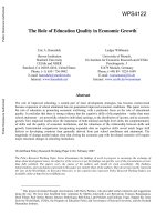
Mean Annual Earnings of Males, Twenty-Five Years and Over by
School Years Completed, Selected Years
School year
1939
1949
1956 1958 1959
1963
1966
Elementary 0—4
$
665
$1,724
$2,127 $2,046
$2,935
$2,465

$2,816
5—6 or 5—7 900
2,268
2,927
2,829
4,058
3,409
3,886
7—8 or 8
1,188
2,693 2,829 3,732
3,769
4,725 4,432
4,896
High School 1—3
1,379 3,226
4,480
4,618 5,379
5,370 6,315
4 1,661
3,784
5,439 5,567
6,132 6,588 7,626
College 1—3
1,931
4,423 6,363 6,966 7,401
7,693
9,058
4+ or 4 2,607 6,179
8,490 9,206 9,255

9,523
11,602
5+ — — — — 11,136 10,487
13,221
NOTE: Earnings
in 1939 and 1959; total income in 1949, 1958, 1963 and 1966.
SOURCE: Columns 1, 2, 3, 4, H.P. MiHer [42, Table 1, p. 9661. Column 5 from 1960 Census of Population,
PC(2)—7B, "Occupation by Earnings and Education." Columns 6 and 7 compute(1 from Current Population Re-
porrs, Series P—60, No. 43 and 53, Table 22 and 4 respectively, using midpoints of class intervals and $44,000
for the over $25,000 class. The total elementary figure in 1940 broken down on the basis of data from the 1940
Census
of
Population. The "less than 8 years" figure in 1949 split on the basis of data given in u.S. llouthakker
[34].
In 1956, 1958, 1959, 1963 and 1966, split on the basis of data on earnings of males 25—64 from the 1959
I-in-a-I 000 Census sample. We are indebted to C. Hanoch [31] for providing us with this tabulation.
".513.
___________________
S
1. Re!
p'
e
alive Prices and Changes in the Distribution of the Labor
Force
p'
e
p'
e
p'
e

p'
e
p'
p'
School
1939
19.10—
Completed
48
19491948—1956
1952—
19581957—
52 57
59
1958
1959—
(12
1963
1962—
65
1966
1965—
67
Elementary
0—4
0.497 —2.3
0.521—0.30.452 —1.3
0.409 —0.8
0.498 —0.8
0.407 —0.8

.38() —0.7
5—6 or 5—7
0.672 —3.1
0.685
—0.5
0.624 —0.2
0.565
—1.0
0.688 —0.9
0.562
—1.5
.525
—0.5
7—8 or 8
0.887 —6.8
0.813
—1.8
0.790 —3.3
0.753 —1.20.801 —1.9
0.731
—1.2 .661
—1.!
High School
1—3
1.030
2.40.974—1.3
0.955
(1.7
0.923
0.6

0.9 12—0.6
0.8s6 —0.3
.861 —01
4
1.241
7.0
1.143
1.0 1.159
2.0
1.113
0.9
1.039
1.6
1.087
3.2
l.03()
tU.s
College
1—3
1.442 1.4 1.336
1.2 1.3560.2
1.392
0.7
1.255
1.3
1.269
0
1.223
1.3
4+ or 4 1.947

1.3 1.866
1.6
l.Sl()
1.3
1.810
0.9
1.569
1.0
l.571
0.2
1.566
0.5
5 + — — — — — — — —
1 .888
0.3
I .130
(1.1
1 .785
0. I
ft. Labor input Per Man: Percentage
Change
1910—48
19.18—52 1952—57
1957—59
1959 62 1962—05
1965—67
'l'otal
6.15
2.50
2.97

2.:9
2.36
2.3
1.77
Annual
0.78
0.62 0.59
1.2(1
0.79
0.72
0.88
TABLE 3
Relative Prices,8 Changes in Distribution of the Labor Force, and Indexes of Labor in
put Per Man,
U.S. Males, Civilian Labor Force, 1940—64
rn
0
C
0
z
z
0
0
0
C
0
z
C
7
-1

0
7
rel at
iv , pricesare
comIute(l
using the appropriatebeginning
pen od (I istri hutien of the labor force'
weights.
SOUIWE:
Derived freji, Iahles
1
ai,1 2.
I
EDUCATION IN PRODUCTION FUNCTIONS AND GROWTH ACCOUNTING
79
the percentage completing high school and more (from 28 in 1940 to
58 in 1967). Table 2 presents data on mean income of males by school
years completed, and Table 3 uses these data together with Table 1 to
derive an estimate of the implied rate of growth of labor input (quality)
per worker.8 The columns in Table 3 come in pairs (for example, the
columns headed 1939 and 1940—48). The first column gives the esti-
relative wage (income) of a particular class and is derived by
expressing the corresponding numbers in Table 2 as ratios to their aver-
age (the average being computed using the corresponding entries of
Table 1
weights). The second column of each pair is derived as the
difference between two corresponding columns of Table 1. It gives the
•
change in percentages of the labor force accounted for by different edu-
•

cational classes. The estimated rate of growth of labor quality during a
•
particular period is then derived simply as the sum of the products of the
two columns, and is converted to per annum units.7
For the period as a whole, the quality of the labor force so corn-
puted grew at approximately 0.8 per cent per year. Since the total share
':
oflabor compensation in GNP during this period was about 0.7, about
0.6 per cent per year of aggregate growth can be associated with this
2
variable, accounting for about one-third of the measured "residual."
•'
A comparison and review of similar estimates for other countries can be
found in Selowsky's [52] dissertation and Denison [18].
Note that in these computations no adjustment was made to the
relative weights for the possible influence of "ability" on these differen-
tials. Also, while a portion of observed growth can be attributed to the
changing educational composition of the labor force, it should not be
2
interpreted
to imply that all of it has been produced by or can be attrib-
uted to the educational system. I shall elaborate on both of these points
later on in this paper.
It is important to note that by using a Divisia type of index with
shifting
weights, one can to a large extent escape the criticism of using
These income figures are deficient in several respects; among others: they are
not standardized for age, and the use of a common $44,000 figure for the "over
$25,000" class probably results in an underestimation of educational earnings dif-
5

ferentials. I am indebted to E. F. Denison for pointing this out to me.
2
7 The percentage change so calculated between any two dates, is the same as
would be obtained by weighting the two educational distributions by the base
(weight) period i
earnings,
aggregating and computing the percentage change.
80
EDUCATION AND PRODUCTION FUNCTIONS
"average" instead of "marginal" rates (or products) to weight the various
education categories. If the return to a particular type of education is
declining, such indexes will pick it up with not too great a lag and read-
just its weights accordingly. Also, note that I have not elaborated on the
alternative of using the growth in "human capital" to construct similar
indexes. For productivity measurement purposes, we want indexes based
on "rental" rather than "stock" values as weights. It can be shown (see
Selowsky [52]),
thatif similar data are used consistently, there is no
operational difference between the quality index described above and a
"human capital times rate of return" approach, provided the capital valu-
ation is made at "market prices" (i.e., based on observed rentals) rather
than at production costs. For my purposes, the construction of "human
capital" series would only add to the "round-aboutness" of the calcula-
tions. Such calculations (or at least the calculation of the rates of return
associated with them) are, of course, required for discussions of; optimal
investment in education programs.
IIIEDUCATION AS A VARIABLE IN
AGGREGATE PRODUCTION FUNCTIONS
MUCH of the criticism of the use of such education per man indexes as
measures of the quality of the labor force is summarized by two related

questions: 1. Does education "really" affect productivity? 2. Is "educa-
tion" and its contribution measured correctly for the purpose at hand?
After all, the measures I have presented are not much more than account-
ing conventions. Evidence (in some casual sense) has yet to be presented
that "education" explains productivity differentials and that, moreover,
the particular form of this variable suggested above does it best. There
•
is, of course, a great deal of evidence that differences in schooling are a
major determinant of differences in wages and income, even holding
many other things constant.8 Also, rational behavior on the part of
employers would lead to the allocation of the labor force in such a way
that the value of the marginal product of the different types of labor will
8See Blaug [6] and Schultz [55]
for
extensive bibliographies on this subject.
IL
EDUCATION IN PRODUCTION FUNCTIONS AND GROWTH ACCOUNTING 81
be roughly proportional to their relative wages. Still, a more satisfactory
way of really nailing down this point, at least for me, is to examine the
role of such variables in econometric aggregate production function
studies. Such studies can provide us with a procedure for "validating"
the various suggested quality adjustments, and possibly also a way of
discriminating between alternative forms and measures of "education."
Consider a very simple Cobb-Douglas type of aggregate production
function:
Y =
AKaLs,
where Y is output, K is a measure of capital services, and L is a measure
of labor input in "constant quality units." Let the correct labor input
measure be defined as

L=EN,
where N is the "unweighted" number of workers and E is an index of
the quality of the labor force. Substituting EN for L in the production
function, we have
Y =
AKaE$N8,
providing us with a way of testing the relevance of any particular can-
•
didate for the role of E. At this level of approximation, if our index of
quality is correct and relevant, when the aggregate production function
is estimated using N and E as separate variables, the coefficient of quality
(E) should both be "significant" in some statistical sense and of the
same order of magnitude as the coefficient of the number of workers (N).9
•
It is this type of reasoning which led me, among other things, to embark
° The E measure as used here is equivalent to the "labor-augmenting technical
change" discussed in much of recent growth literature. I prefer, however, to interpret
•
it as an approximation to a more general production function based on a number
of different types of labor inputs. Allowing changing weights in the construction of
such an E index implicitly allows for a very general production function (at least
over the subset of different L types) and imposes very few restrictions on it. An
interpretation of E as an index of embodied quality in different types and vintages
of labor, fixed once and for all and independent of levels of K, would be very
restrictive and is not necessary at this level of aggregation.
• I

—
82 EDUCATION
AND PRODUCTION

FUNCTIONS
TABLE 4
Education and Skill Variables in Aggregate
Production Function Studies
Industry, Unit of
Observation Period
and Sample Size
Labor
Coefficient
Education or
Skill Variable
Coefficient
R2
1.
U.S. Agriculture,
68 Regions, 1949 a 45 .977
(.07)
b 52
(.08)
.43
(.18)
.979
2.
U.S. Agriculture,
39 "states," 1949—
54—5 9 a.
.43
.980
(.05)
b 51

(.06)
.41
(.16)
.981
3.
U.S. Manufacturing,
states and two—digit
industries, N=4 17,
1958
a.
.67
.547
(.0 1)
b.
.69
(.01)
.95
(.07)
.665
4.
U.S. Manufacturing,
states and two—digit
industries, N=783,
1954—57—63 a.
.71
.623
(.01)
b.
.75
(.01)

c 85
(.01)
.96
(.06)
.56
(.16)
.757
.884
NOTE: All the variables (except for state industry, or time dummy
variables) are in the form of logarithms of original values. The numbers
I
I
•1
''I
—p
EDUCATION IN
PRODUCTION FUNCTIONS AND GROWTH
83
in parentheses are the calculated standard errors of the respective
coefficients.
SOURCES:1.
Griliches [231, TableI. Dependent variable: sales,
home consumption, inventory change, and government payments. Labor:
full-time equivalent man-years. "Education'' — average education of
the rural farm population weighted by average income by education
class-weights for the U.S. as a whole, per man. Other variables in-
cludedinthe regression: livestock inputs, machinery inputs, Land,
buildings, and other current inputs. All variables (except education)
are averages per commercial farm in a region. 2. Griliches [24], Table 2.
Dependent variable: same as

in
(I) but deflatedfor price change.
S
Labor:
total man—days, with downward adjustments for operators over
65 and unpaid family workers. Education: sirtdlar to
(1). Other var-
iables: Machinery inputs, Land and buildings, Fertilizer, "Other", and
time dummies. All of the variables (except education and the time
•
dummies) are per farm state averages.
3.
Griliches [25], Table 5.
Dependent variable: Value added per man-hour. Labor: total man-hours.
Skill: Occupational mix-annual average income predicted for the partic-
ular
labor force on the basis of its occupational mix and national
average incomes by occupation. Other variable: Capital Services. All
variables in per-establishment units. 4. Griliches [27], Table 3. De-
pendent, labor, and skill variables same as above. Other variables: a.
and b. Capital based on estimated gross-book-value of fixed assets;
c. also includes 18 Industry and 20 regional dummy variables.
on
a series
ofeconometric production function studies using regional data
for U. S. agriculture and manufacturing industries. The results of these
studies, as far as they relate to the quality of labor variables, are sum-
marized in Table 4.'°
In general they support the relevance of such "quality" variables
fairly well. The education or skill variables are "significant" at conven-

tional statistical levels and their coefficients are, in general, of the same
order of magnitude (not "significantly" different from) as the coefficients
of the conventional labor input measures. It is only fair to note that the
•
inclusion
of education variables in the agricultural studies does not
4
•
10
data
sources andmanycaveats are described in detail in the original
articles cited in Table 4 and will not be reproduced here. Note that for manufactur-
•
ing, the quality variable is based on an occupation-by.industry rather than education-
•
by-industry distribution, since the latter was not available at the state level. On
the other hand, the first manufacturing study (Griliches [25])alsoexplored the
influence of age, sex, and race differences on productivity, topics which will not be
pursued further here.
84
EDUCATION AND PRODUCTION FUNCTIONS
increase greatly the explained variance of output per farm at the cross-
sectional level, while the expected equality of the coefficients of E and N
is only very approximate in the manufacturing studies. Nevertheless, this
is about the only direct and reasonably strong evidence on the aggregate
productivity of "education" known to me, and I interpret it as supporting
both the relevance of labor quality so measured and the particular way
of measuring it."
There have been a few attempts to introduce education variables in
a different way. Hildebrand and Liu [33] considered the possibility that

an education variable may modify the exponent of a conventional mea-
sure of labor in a Cobb-Douglas type production function. Their empiri-
cal results, however, did not provide any support for such a hypothesis,
partly because of lack of relevant data. They used the education of the
total labor force in a state for the measurement of the quality of the
labor force of individual industries within the same state. But the diffi-
culty of estimating interaction terms of the form E log L implied by their
hypothesis, arises mostly, I believe, because there is no good theoretical
reason to expect this particular hypothesis (that education affects the
share of labor in total production) to be true. Brown and Conrad [13]
have proposed the more general (and hence to some extent emptier)
hypothesis that education affects all the parameters of the production
function. They did not, however, estimate a production function directly,
including instead a measure of the median years of schooling in ACMS
type of time series regressions of value added per worker on wage rates
and other variables. Their results are hard to interpret, in part because
their education variables are fundamentally trends (having been inter-
polated between the observed 1950 and 1960 values), and because the
same final equation is implied by the very much simpler errors-in-the-
measurement of labor model. Nelson and Phelps [46] have suggested that
education may affect the rate of diffusion of new techniques more than
their level. This would imply in cross-sectional data that education affects
the over-all efficiency parameter instead of serving as a modifier of the
labor variable. Nelson and Phelps do not present any empirical estimates
of their model. Without further detailed specification of their hypothesis,
it is not operationally different from the quality of labor view of educa-
11 Somewhat similar results have also been reported by Besen [5].
EDUCATION IN PRODUCTION FUNCTIONS AND GROWTH ACCOUNTING- 85
tion in a Cobb-Douglas world, since any multiplicative variable can
always be viewed as modifying the constant instead of one of the other

variables.'2
No studies, as far as I know, have used a human capital variable as
an alternative to the labor-augmenting quality index in estimating pro-
duction functions. While at the national accounting level
it need not
make any difference which variable is used, the two approaches used in
a Cobb-Douglas framework would imply different elasticities of substi-
tution between different types or components of labor. Consider two
alternative aggregate production function models
Y =
= AKaN$E$
where E =
and the ri's are some base period rentals (wages)
for the different categories of labor, and
Y =
where H is a measure of "human capital." To be consistent with the E
measure it would have to be based on a capitalization of the wage differ-
entials over and above the returns to "raw," unskilled, or uneducated
labor (r0)
Thus, approximately
H =
(r1 —
where
is a capitalization ratio on the order of one over the discount
rate. Note, that given our definitions we can rewrite H as
H = ö(EN —roN)
ÔN(E —
rç,)
12 Data from the 1964 Census of Agriculture may allow a test of the Nelson-
Phelps hypothesis. These data provide separate information on the education of

the farm operator
as
distinct from that of the rest of the farm labor force. The
• Nelson-Phelps hypothesis implies that the education of entrepreneurs is a more
crucial, in some sense, determinant of productivity than the education of the rest
•
of the labor force.
13 An H index based on costs (income forgone and the direct costs of schooling)
would be similar to the one described in the text only if all rates of return to dif-
ferent levels of education were equal to each other and to the rate used in the con-
struction of the human capital estimate.
Education
Variable
Coefficients of
R2
X6
(man-years)
Education
Variable
S
.539
.0165
(.0065)
.9789
log S
.536
.297
(.119)
.9789
E

.524
.431
(.181)
.9787
E2
.520 .455
(.203)
.9785
S—Mean school years completed of the rural
farm population (25
years
old and over). E—Logarithm of
theschool
years completed
distribution of the rural farm population weighted by mean income of
all
U.S. males, 25 years and over in1949. Mean incomes from H.
Houthakker [34]. E2—Same as E except that the weights are mean
wage and salary income of native white males (over 25)
in1939.
Mean incomes by school years completed computed from the 1940
Census of Population, Education, Washington, 1947, pp. 147 and 190.
Other variables are the same as in row
1 of Table 4.
SOURCE: Unpublished mimeographed appendix
to
Griliches [23].
and substituting it into the human capital version of the production func-
tion we get
Y

(i —
Thus, the H version implies that the production function written in terms
of E is not homothetic with respect to E. Moreover, it implies that the
elasticity of substitution between H and N is unity, while the E version
assumes (for fixed r's) that the elasticity of substitution between different
-
86.EDUCATION
AND PRODUCTION FUNCTIONS
TABLE 5
Various Education Measures in an Aggregate
Agricultural Production Function
(Sixty-Eight Regions, U.S. 1949)
I
I
—P
EDUCATION IN PRODUCTION FUNCTIONS AND GROWTH ACCOUNTING
87
types of labor (the N,) is infinite, at least in the neighborhood of the
observed price ratios.
While such different assumptions are not operationally equivalent,
it is probably impossible to discriminate between them on the basis of
the type and amounts of data currently available to us. Consider the last
equation; it differs from the straight E version by having a different
coefficient on E than on N. If we estimate the E equation in an H world,
we shall be leaving out the variable log(1 —
r0/E)with a c coefficient in
front of it. But log(l —
r0/E)
is approximately equal to —r0/E, since
r0/E < 1, and the regression coefficient of the left out variable, in the

form of 1 /E on the included variable log E, will be on the order of one,
for not too large variations in E. Hence, the estimated coefficient of E in
•
an H world will be on the order of 2c, which is not likely to be too dif-
• ferent from the coefficient of
More generally, it
is probably impossible to distinguish between
various different but similar hypotheses about how the index E should be
measured, at least on the basis of the kind of data I have had access to.
•
Whether
one uses "specific" or national income weights, or just simply
the average number of school years completed, one has variables that are
very highly correlated with each other. This is illustrated by the results
reported in Table 5, based on an unpublished appendix to my 1963
study. Our data are just not good enough to discriminate between "fine"
hypotheses about the form (curvature) of the relationship or the way in
which such a variable is to be measured.
•
IV
AGGREGATION
OBVIOUSLY, in constructing such indexes of "quality" (or human capital)
we are engaged in a great deal of aggregation. There are many different
types and qualities of "education" and much of the richness and the
mystery of the world is lost when all are lumped into one index or num-
ber. Nevertheless, as long as we are dealing with aggregate data and ask-
ing over-all questions, the relevant consideration is not whether the under-
lying world is really more complex than we are depicting it, but rather
whether that matters for the purpose of our analysis. And even if we
. —

Year
High School
Elementary
Graduates to
-,
SchoolGrads
College Graduates to
.
High
School Graduates
1939
1949
140a
1.41
134b
157C
1.63
1958
1959
1.48
1.30
1.65
1•51d
1963
1.49 1.45
1966 1.56
1.52
aElementary 7—8
years
bElementary

8 years
CColIege 4
+ years
dColiege
4 years
SOURCE: From Table 3
decide that one index of E hides more than it reveals, our response will
surely not be "therefore let's look at 23 or 119 separate labor or educa-
tion categories," but rather what kind of two-, three-, or four-way dis-
aggregation of E will give us the most insight into the problem.
From a formal point of view, we can appeal either to the Hicks
composite-good or to the Leontief separability theorems to guide us in
the quest for correct aggregation. If relative prices (rentals or wages) of
labor with different schooling or skill levels have remained constant, then
we lose little in aggregating them into one composite input measure.
A glance at the "relative prices" for different educational classes reported
for the United States in Table 3 does not reveal any drastic changes in
them. Thus, it is unlikely that at this level of aggregation much violence
is done to the data by putting them further together into one L or E
index. Similar results can be gleaned from a variety of occupational and
skill differential data (see Tables 6 and 7). In general, they have re-
mained remarkably stable in the face of very large changes in relative
k.
.7
88
.EDUCATION
AND PRODUCTION FUNCTIONS
TABLE 6
Ratios of Mean Incomes for U.S. Males
by Schooling Categories

I.
i
1947 1.67
1950
1.58
1953 1.55
1959 1.67
1964
1.63
SOURCE: From U.S. Bureau of Census, Trends in Income of Fam-
ilies and Persons in the U.S.: 1947 —
1964,Technical Paper No. 17,
Washington, 1967, Table 38.
numbers and other aspects of the economy.'4 In fact, the apparent con-
stancy of such numbers constitutes a major economic puzzle to which
I shall come back later.
When we abandon the notion of one aggregate labor input and are
faced with a lis.t of eight major occupations, eight schooling classes, sev-
eral regions, two sexes, at least two races, and an even longer list of
detailed occupations, there doesn't seem to be much point in trying to dis-
tinguish all these aspects of the labor force simultaneously. The next small
step is obviously not in the direction
a very large number of types of
labor but rather toward the question of whether there are a few under-
lying relevant "dimensions" of "labor" which could explain, satisfac-
torily, the observed diversity in the wages paid to different "kinds" of
labor. The obvious analogy here is to the hedonic or characteristics
approach to the analysis of quality change in consumer goods, where an
attempt is made to reduce the observed diversity of "models" to a smaller
set of relevant characteristics such as size, power, durability, and so

forth.'5 One can identify the "human capital" approach as a one-dimen-
14 The constancy of relative differentials implies a rise in absolute differential and
a rise in the incentive to individuals to invest more in their education.
15 See Griliches [261 and Lancaster (411 for a recent survey and exposition of such
an approach.
EDUCATION IN PRODUCTION FUNCTIONS AND GROWTH ACCOUNTING
. 89
TABLE
7
Ratios of Mean Incomes of U.S. Employed and Salaried Males:
Professional and Technical Workers to Operatives and Kindred
Year
4.
90
EDUCATION AND PRODUCTION FUNCTIONS
sional version of such an approach.16 Each person is thought of as con-
sisting of one unit of raw labor and some particular level of embodied
human capital. Hence, the wage received by such a person can be viewed
as the combination of the market price of "bodies" and the rental value
of units of human capital attached to (embodied in) that body:
w, =w0
+ rH, +
where u4 stands for all other relevant characteristics (either included
explicitly as variables, controlled by selecting an appropriate sub-class,
or assumed to be random and hence uncorrelated with He). If direct esti-
mates of H are available, this type of framework can be used to estimate
r. If proxy variables are used for H, such as years of schooling, age, or
"experience," one can proceed to the estimation of income-generating
functions as did Hanoch [31] and Thurow [59] which, in turn, can be
interpreted as "hedonic" regressions for people. Alternatively, if one is

willing to assume that the implicit prices (w0 and r) are constant, and
one has repeated observations for a given i, one can use such a frame-
work to estimate the unobserved "latent" variable. Consider, for
example, a sample of wages by occupation for different industries: If one
assumes that occupations differ only by the amount of human capital
embodied per capita, and that the price of "bodies" and of "skill" is
equalized across industries, then this is just a one-factor analysis model,
and it can be used to estimate the implied relative levels of
for differ-
ent occupations. Of course, having gone so far one need not stop at one
factor, or only one underlying skill dimension. The question can be
pushed further to how many latent factors or dimensions are necessary
or adequate for an explanation of the observed differences in wages
across occupations and schooling classes?
This is, in fact, the approach pursued by Mitchell [44] in analyzing
the variation of the average wage in manufacturing industries by states.
He concludes that one "quality" dimension is enough for his purposes.
He does, however, make the very stringent assumption that the implied
16 Actually, it could be thought of as a two-dimensional or factors model, body
and skill, but since each person is taken to have only one unit of body (even a
Marilyn Monroe), the B
dimensionbecomes a numeraire and for practical purposes
this reduces itself to a one-factor model.
4
EDUCATION IN PRODUCTION FUNCTIONS AND GROWTH ACCOUNTING
91
relative
price ratio of bodies to human capital, or of skilled and unskilled
wages (w0/r),
is

constant across states and countries. This is a very
strong assumption, one that is unlikely to be true for data cross-classified
by schooling. Studies of U. S. data (see, e.g., Welch, [62] and Schwartz
[511 have in general found significantly more regional variation in the
price of unskilled or uneducated labor than in the price of skilled or
highly educated labor, implying the nonconstancy of skill differentials
across regions (and presumably also countries).
In a recent paper, Welch [63] outlines a several dimensions model
of the general form
w,,
= w01 +
+ r27S21
where i is the index for the level of school years completed, jis
the index
for states,
and S2 are two unobserved underlying skill components
associated with different educational levels. This is not strictly a factor-
analysis model any longer, both because the r's are assumed to vary
across states and because no orthogonality assumptions are made about
the two latent skill levels. With a few additional assumptions, Welch
shows that if the model is correct one should be able to explain the wage
of a particular educational or skill level by a linear combination of wages
for other skill levels and by no more than three such wages (since there
are only three prices here: two "skills" and one "body"). The linearity
arises from the implicit assumption that at given prices any unit of S1 or
S2 (and "body") is a perfect substitute for another. Thus, even though
•
different types of labor are made up of a smaller number of different
qualities which may not be perfectly substitutable for each other, because
the whole bundle is defined linearly, one can find linear combinations of

several types of labor which will be perfectly substitutable for another
type of labor. For example, while college and high school graduates may
not be perfect substitutes, one college graduate plus one elementary
school graduate may be perfect substitutes for two high school graduates.
Welch analyzes incomes by education by states and concludes that in
general one doesn't need more than three underlying dimensions to
explain eight observed wage levels, and that often two are enough. It is
•
not clear whether Welch is using the best possible and most parsimonious
normalization, or whether a generalization of the factor-analytic approach
92
EDUCATION AND PRODUCTION FUNCTIONS
with oblique factors could not be adapted to this problem, but clearly
this is a very interesting and promising line of analysis.
The approximate constancy of relative labor prices by type, the
implicit linearity of the Welch model, and some scattered estimates of
rather high elasticities of substitution between different kinds of labor or
education levels (e.g., Bowles [8]), all imply that we will lose little by
aggregating all the different types of labor into one over-all index as long
as our interest is not primarily in the behavior of these components and
their relative prices.
V
ABILITY
THIS is a very difficult topic with a large literature and very little data.
What little relevant data there are have been recently surveyed by Becker
[2] and Denison [17]. It has been widely suggested that the usual income-
by-education figures overestimate the "pure" contribution of education
because of the observed correlation between measured ability and years
of school completed. On the basis of scattered evidence both Becker and
Denison decide to adjust downward the observed income-by-education

differentials, Denison suggesting that all differentials should be reduced
by about one-third.
It is useful, at this point, to set up a littLe model to help clarify the
issues. Assume that the true relation in cross-sectional data is
Y
is income, sis
schooling and A is ability, however measured.
The usual calculation of an income-schooling relation alone leads to an
estimate of a schooling coefficient (br,) whose expected value is higher
than the true "net" coefficient of schooling (J31), as long as the correlation
between schooling and the left out ability variable is positive. The exact
bias is given by the following formula:
=
+ f32bAs
where bAa is the regression coefficient in the (auxiliary) regression of
k
.7
EDUCATION IN PRODUCTION FUNCTIONS AND GROWTH ACCOUNTING• 93
the
left out variable A On 5, the included one. Moving to time series now,
and still assuming that the underlying parameters
and /32) do not
change, we have the relationship
=
/3o
+
/31S + /3214 +
U
where
the bars stand for averages in a particular year. Now if is

derived from cross-sectional data and is used in conjunction with the
change in the average schooling level to predict (or explain) changes in
Y over time, it will overpredict them (give too high a weight to
unless A changes pan passu. But it is assumed that the distribution of A,
innate ability,
is fixed over time and hence, its mean (A) does not
change.This,
therefore,
isthe rationale for considering the cross-
sectional income-education weights with some suspicion and for adjusting
them downward for the bias caused by the correlation of schooling with
ability.
I should like to question these downward adjustments on three
related grounds: 1. Much of measured ability is the product of "learn-
ing," even if it is not all a product of "schooling." Often what passes for
"ability" is actually some measure of "achievement," and the argument
could be made that it in turn is determined by a relation of the form
A a0+a1S+a2QS+a3LH+a4G+v
where S is the level of schooling, QS is the quality of schooling, LH are
the learning inputs at "home," and G is the original genetic endowment.
If one were to substitute this equation into the original relation for Y
one would find that the "total" coefficient of the schooling variables is
given by
£
+f32a1+f32a2bQs.s
where bQ3.3 is the relation between the quality and quantity of schooling
in the cross-sectional data, and the "total" coefficient associated with
changes in total "reproducible" human capital (including that produced
at home) by
+ /32 I

a,+
+ a3bLJf.8 I
where
bLH.8 summarizes the relation between learning at home and at
94
EDUCATION AND PRODUCTION FUNCTIONS
school in cross-section. Now while the simple coefficient of income and
schooling may
overestimate the partial effect of schooling (f3i) hold-
ing achievement constant, it may not overestimate that much, if at all,
the "total" effect of schooling. 2. The estimated downward adjustments
for ability may be overdone particularly in the light of strong interaction
of "ability" and schooling as they affect earnings. That is, since the rela-
tion between A and Y holding S constant is strong only at higher S levels,
b43 may be quite low, and the bias in the estimated
may not be all
that large. 3. Moreover, the whole issue hinges on whether or not A as
measured has really remained constant over time. To the extent that
proxies such as father's education are used in lieu of "ability," it can be
shown that at least their levels did not remain constant.
It is probably best, at this point, to confess ignorance. "Ability,"
"intelligence," and "learning" are all very slippery concepts. Nor do we
know much about the technology of schooling or education. What are
the important inputs and outputs, whal is the production function of
education, how do the various inputs interact? Some work on this is in
progress (see Bowles [9]) and perhaps we will know more about it in the
future. We do know, however, the following things: 1. Intelligence is not
a fixed datum independent of schooling and other environmental influ-
ences. 2. It can be affected by schooling.17 3. It in turn affects the amount
of learning achieved in a given schooling situation. 4. Because the scale

in which it is measured is arbitrary, it is not clear whether the relative
distribution of "intelligence" or "learning abilities" has remained con-
stant over time.
The doctrine that intelligence is a unitary something that is estab-
lished for each person by heredity and that stays fixed through life
should be summarily banished. There is abundant proof that greater
intelligence is associated with increased education Onthe basis
of present information it would be best to regard each intellectual
•
ability of a person as a somewhat generalized skill that has devel-
oped through the circumstances of experience, within a certain cul-
• ture, and that can be further developed by means of the right kind
•
of exercise. There may be limits to ability set by heredity, but it is
probably safe to say that very rarely does an individual really test
¶
such ljmjts18
iT See e.g., the studies of separated identical twins summarized in Bloom [7J.
18 Guilford [28],
p.
619.
I —

•