Higher-Order Perl pdf
Bạn đang xem bản rút gọn của tài liệu. Xem và tải ngay bản đầy đủ của tài liệu tại đây (1.91 MB, 592 trang )
Praise for Higher-Order Perl
As a programmer, your bookshelf is probably overflowing with books that did nothing to change the way you
program orthink about programming.
You’re going to need a completely different shelf for this book.
While discussing caching techniques in Chapter 3, Mark Jason Dominus points out how a large enough
increase in power can change the fundamental way you think about a technology. And that’s precisely what
this entire book does for Perl.
It raids the deepest vaults and highest towers of Computer Science, and transforms the many arcane treasures
it finds—recursion, iterators, filters, memoization, partitioning, numerical methods, higher-order functions,
currying, cutsorting, grammar-based parsing, lazy evaluation, and constraint programming—into powerful
and practical tools for real-world programming tasks: file system interactions, HTML processing, database
access, web spidering, typesetting, mail processing, home finance, text outlining, and diagram generation.
Along the way it also scatters smaller (but equally invaluable) gems, like the elegant explanation of the
difference between “scope” and “duration” in Chapter 3, or the careful exploration of how best to return
error flags in Chapter 4. It even has practical tips for Perl evangelists.
Dominus presents even the most complex ideas in simple, comprehensible ways, but never compromises on
the precision and attention to detail for which he is so widely and justly admired.
His writing is—as always—lucid, eloquent, witty, and compelling.
Aptly named, this truly /is/ a Perl book of a higher order, and essential reading for every serious Perl
programmer.
—Damian Conway, Co-designer of Perl 6-
-
Mark Jason Dominus
AMSTERDAM • BOSTON • HEIDELBERG • LONDON
NEW YORK • OXFORD • PARIS • SAN DIEGO
SAN FRANCISCO • SINGAPORE • SYDNEY • TOKYO
Morgan Kaufmann Publishers is an imprint of Elsevier
Senior Editor Tim Cox
Publishing Services Manager Simon Crump
Assistant Editor Richard Camp
Cover Design Yvo Riezebos Design
Cover Illustration Yvo Riezebos Design
Composition Cepha Imaging Pvt. Ltd.
Technical Illustration Dartmouth Publishing, Inc.
Copyeditor Eileen Kramer
Proofreader Deborah Prato
Interior Printer The Maple-Vail Book Manufacturing Group
Cover Printer Phoenix Color
Morgan Kaufmann Publishers is an imprint of Elsevier.
500 Sansome Street, Suite 400, San Francisco, CA 94111
This book is printed on acid-free paper.
© 2005 by Elsevier Inc. All rights reserved.
Designations used by companies to distinguish their products are often claimed as trademarks or
registered trademarks. In all instances in which Morgan Kaufmann Publishers is aware of a claim,
the product names appear in initial capital or all capital letters. Readers, however, should contact
the appropriate companies for more complete information regarding trademarks and registration.
No part of this publication may be reproduced, stored in a retrieval system, or transmitted in any form
or by any means—electronic, mechanical, photocopying, scanning, or otherwise—without prior written
permission of the publisher.
Permissions may be sought directly from Elsevier’s Science & Technology Rights Department in Oxford,
UK: phone: (+44) 1865 843830, fax: (+44) 1865 853333, e-mail: You may
also complete your request on-line via the Elsevier homepage () by selecting
“Customer Support” and then “Obtaining Permissions.”
Library of Congress Cataloging-in-Publication Data
Application submitted
ISBN: 1-55860-701-3
For information on all Morgan Kaufmann publications,
visit our Web site at www.mkp.com or www.books.elsevier.com
Printed in the United States of America
0506070809 54321
For Lorrie
Preface
xv
Recursion and Callbacks 1
1.1
1
1.2
3
1.2.1 Why Private Variables Are Important
5
1.3
6
1.4
12
1.5
16
1.6 -
25
1.7
26
1.7.1 More Flexible Selection
32
1.8
33
1.8.1 Fibonacci Numbers
33
1.8.2 Partitioning
35
Dispatch Tables 41
2.1
41
2.1.1 Table-Driven Configuration
43
2.1.2 Advantages of Dispatch Tables
45
2.1.3 Dispatch Table Strategies
49
2.1.4 Default Actions
52
2.2
54
2.2.1 HTML Processing Revisited
59
Caching and Memoization 63
3.1
65
3.2
66
3.2.1 Static Variables
67
3.3
68
3.4
69
ix
x
3.5
70
3.5.1 Scope and Duration
71
Scope
72
Duration
73
3.5.2 Lexical Closure
76
3.5.3 Memoization Again
79
3.6
80
3.6.1 Functions Whose Return Values Do Not Depend on Their
Arguments
80
3.6.2 Functions with Side Effects
80
3.6.3 Functions That Return References
81
3.6.4 A Memoized Clock?
82
3.6.5 Very Fast Functions
83
3.7
84
3.7.1 More Applications of User-Supplied Key
Generators
89
3.7.2 Inlined Cache Manager with Argument Normalizer
90
3.7.3 Functions with Reference Arguments
93
3.7.4 Partitioning
93
3.7.5 Custom Key Generation for Impure Functions
94
3.8
96
3.8.1 Memoization of Object Methods
99
3.9
100
3.10
101
3.11
108
3.12
109
3.12.1 Profiling and Performance Analysis
110
3.12.2 Automatic Profiling
111
3.12.3 Hooks
113
Iterators 115
4.1
115
4.1.1 Filehandles Are Iterators
115
4.1.2 Iterators Are Objects
117
4.1.3 Other Common Examples of Iterators
118
4.2
119
4.2.1 A Trivial Iterator:
upto() 121
Syntactic Sugar for Manufacturing Iterators
122
4.2.2
dir_walk() 123
4.2.3 On Clever Inspirations
124
xi
4.3 126
4.3.1 Permutations
128
4.3.2 Genomic Sequence Generator
135
4.3.3 Filehandle Iterators
139
4.3.4 A Flat-File Database
140
Improved Database
144
4.3.5 Searching Databases Backwards
148
A Query Package That Transforms Iterators
150
An Iterator That Reads Files Backwards
152
Putting It Together
152
4.3.6 Random Number Generation
153
4.4
157
4.4.1
imap() 158
4.4.2
igrep() 160
4.4.3
list_iterator() 161
4.4.4
append() 162
4.5
163
4.5.1 Avoiding the Problem
164
4.5.2 Alternative
undefs
166
4.5.3 Rewriting Utilities
169
4.5.4 Iterators That Return Multiple Values
170
4.5.5 Explicit Exhaustion Function
171
4.5.6 Four-Operation Iterators
173
4.5.7 Iterator Methods
176
4.6
177
4.6.1 Using
foreach to Loop Over More Than One Array 177
4.6.2 An Iterator with an
each-Like Interface 182
4.6.3 Tied Variable Interfaces
184
Summary of
tie 184
Tied Scalars
185
Tied Filehandles
186
4.7 :
187
4.7.1 Pursuing Only Interesting Links
190
4.7.2 Referring URLs
192
4.7.3
robots.txt 197
4.7.4 Summary
200
From Recursion to Iterators 203
5.1
204
5.1.1 Finding All Possible Partitions
206
xii
5.1.2 Optimizations
209
5.1.3 Variations
212
5.2
215
5.3
225
5.4
229
5.4.1 Tail-Call Elimination
229
Someone Else’s Problem
234
5.4.2 Creating Tail Calls
239
5.4.3 Explicit Stacks
242
Eliminating Recursion From
fib() 243
Infinite Streams 255
6.1
256
6.2
257
6.2.1 A Trivial Stream:
upto() 259
6.2.2 Utilities for Streams
260
6.3
263
6.3.1 Memoizing Streams
265
6.4
269
6.5
272
6.5.1 Generating Strings in Order
283
6.5.2 Regex Matching
286
6.5.3 Cutsorting
288
Log Files
293
6.6 -
300
6.6.1 Approximation Streams
304
6.6.2 Derivatives
305
6.6.3 The Tortoise and the Hare
308
6.6.4 Finance
310
6.7
313
6.7.1 Derivatives
319
6.7.2 Other Functions
320
6.7.3 Symbolic Computation
320
Higher-Order Functions and Currying
325
7.1
325
7.2 -
333
7.2.1 Automatic Currying
335
7.2.2 Prototypes
337
Prototype Problems
338
xiii
7.2.3 More Currying 340
7.2.4 Yet More Currying
342
7.3
reduce() combine() 343
7.3.1 Boolean Operators
348
7.4
351
7.4.1 Operator Overloading
356
Parsing 359
8.1
359
8.1.1 Emulating the
<> Operator 360
8.1.2 Lexers More Generally
365
8.1.3 Chained Lexers
368
8.1.4 Peeking
374
8.2
376
8.2.1 Grammars
376
8.2.2 Parsing Grammars
380
8.3 -
384
8.3.1 Very Simple Parsers
384
8.3.2 Parser Operators
386
8.3.3 Compound Operators
388
8.4
390
8.4.1 A Calculator
400
8.4.2 Left Recursion
400
8.4.3 A Variation on
star() 408
8.4.4 Generic-Operator Parsers
412
8.4.5 Debugging
415
8.4.6 The Finished Calculator
424
8.4.7 Error Diagnosis and Recovery
427
Error-Recovery Parsers
427
Exceptions
430
8.4.8 Big Numbers
435
8.5
435
8.6
440
8.7 -
448
8.7.1 The Lexer
448
8.7.2 The Parser
451
8.8
456
8.8.1 Continuations
457
8.8.2 Parse Streams
461
8.9
465
xiv
Declarative Programming 471
9.1
472
9.2
472
9.2.1 Implementing a Local Propagation Network
475
9.2.2 Problems with Local Propagation
487
9.3
488
9.4
linogram: 490
9.4.1 Equations
500
ref($base) || $base
501
Solving Equations
502
Constraints
512
9.4.2 Values
514
Constant Values
516
Tuple Values
518
Feature Values
520
Intrinsic Constraints
521
Synthetic Constraints
522
Feature-Value Methods
527
9.4.3 Feature Types
530
Scalar Types
531
Type Methods
532
9.4.4 The Parser
539
Parser Extensions
541
%TYPES 542
Programs
543
Definitions
543
Declarations
545
Expressions
554
9.4.5 Missing Features
560
9.5
563
Index 565
Function Index 575
A well-known saying in the programming racket is that a good Fortran pro-
grammer can write Fortran programs in any language. The sad truth, though,
is that Fortran programmers write Fortran programs in any language whether
they mean to or not. Similarly, we, as Perl programmers, have been writing C
programs in Perl whether we meant to or not. This is a shame, because Perl is
a much more expressive language than C. We could be doing a lot better, using
Perl in ways undreamt of by C programmers, but we’re not.
How did this happen? Perl was originally designed as a replacement for C
on the one hand and Unix scripting languages like Bourne Shell and
awk on
the other. Perl’s first major proponents were Unix system administrators, people
familiar with C and with Unix scripting languages; they naturally tended to write
Perl programs that resembled C and
awk programs. Perl’s inventor, Larry Wall,
came from this sysadmin community, as did Randal Schwartz, his coauthor on
Programming Perl, the first and still the most important Perl reference work.
Other important early contributors include Tom Christiansen, also a C-and-
Unix expert from way back. Even when Perl programmers didn’t come from the
Unix sysadmin community, they were trained by people who did, or by people
who were trained by people who did.
Around 1993 I started reading books about Lisp, and I discovered something
important: Perl is much more like Lisp than it is like C. If you pick up a good
book about Lisp, there will be a section that describes Lisp’s good features.
For example, the book Paradigms of Artificial Intelligence Programming, by Peter
Norvig, includes a section titled What Makes Lisp Different? that describes seven
features of Lisp. Perl shares six of these features; C shares none of them. These
are big, important features, features like first-class functions, dynamic access to
the symbol table, and automatic storage management. Lisp programmers have
been using these features since 1957. They know a lot about how to use these
language features in powerful ways. If Perl programmers can find out the things
that Lisp programmers already know, they will learn a lot of things that will make
their Perl programming jobs easier.
This is easier said than done. Hardly anyone wants to listen to Lisp pro-
grammers. Perl folks have a deep suspicion of Lisp, as demonstrated by Larry
Wall’s famous remark that Lisp has all the visual appeal of oatmeal with fingernail
xv
xvi
clippings mixed in. Lisp programmers go around making funny noises like ‘cons’
and ‘cooder,’ and they talk about things like the PC loser-ing problem, whatever
that is. They believe that Lisp is better than other programming languages, and
they say so, which is irritating. But now it is all okay, because now you do not
have to listen to the Lisp folks. You can listen to me instead. I will make sooth-
ing noises about hashes and stashes and globs, and talk about the familiar and
comforting soft reference and variable suicide problems. Instead of telling you
how wonderful Lisp is, I will tell you how wonderful Perl is, and at the end you
will not have to know any Lisp, but you will know a lot more about Perl.
Then you can stop writing C programs in Perl. I think that you will find it
to be a nice change. Perl is much better at being Perl than it is at being a slow
version of C. You will be surprised at what you can get done when you write Perl
programs instead of C.
All the code examples in this book are available from my web site at:
/>When the notation in the margin is labeled with the tag some-example, the
code may be downloaded from:
/>The web site will also carry the complete text, an errata listing, and other items
of interest. Should you wish to send me email about the book, please send your
message to
Every acknowledgments section begins with a statement to the effect that “with-
out the untiring support and assistance from my editor, Tim Cox, this book
would certainly never have been written”. Until you write a book, you will never
realize how true this is. Words fail me here; saying that the book would not
have been written without Tim’s untiring support and assistance doesn’t begin
to do justice to his contributions, his kindness, and his vast patience. Thank
you, Tim.
xvii
This book was a long time in coming, and Tim went through three assistants
while I was working on it. All these people were helpful and competent, so my
thanks to Brenda Modliszewksi, Stacie Pierce, and Richard Camp. “Competent”
may sound faint, but I consider it the highest praise.
Many thanks to Troy Lilly and Simon Crump, the production managers,
who were not only competent but also fun to work with.
Shortly before the book went into production, I started writing tests for the
example code. I realized with horror that hardly any of the programs worked
properly. There were numerous small errors (and some not so small), inconsis-
tencies between the code and the output, typos, and so on. Thanks to the heroic
eleventh-hour efforts of Robert Spier, I think most of these errors have been
caught. Robert was not only unfailingly competent, helpful, and productive,
but also unfailingly cheerful, too. If any of the example programs in this book
work as they should, you can thank Robert. (If they don’t, you should blame
me, not Robert.) Robert was also responsible for naming the MOD document
preparation system that I used to prepare the manuscript.
The contributions of my wife, Lorrie Kim, are too large and pervasive to
note individually. It is to her that this book is dedicated.
A large number of other people contributed to this book, but many of them
were not aware of it at the time. I was fortunate to have a series of excellent
teachers, whose patience I must sometimes have tried terribly. Thanks to Mark
Foster, Patrick X. Gallagher, Joan Livingston, Cal Lobel (who first taught me to
program), Harry McLaughlin, David A. J. Meyer, Bruce Piper, Ronnie Rabassa,
Michael Tempel, and Johan Tysk. Mark Foster also arrived from nowhere in the
nick of time to suggest the title for this book just when I thought all was lost.
This book was directly inspired by two earlier books: ML for the Working
Programmer, by Lawrence Paulson, and Structure and Interpretation of Computer
Programs, by Harold Abelson and Gerald Jay Sussman. Other important influ-
ences were Introduction to Functional Programming, by Richard Bird and Philip
Wadler, and Paradigms of Artificial Intelligence Programming, by Peter Norvig.
The official technical reviewers had a less rewarding job than they might have
on other projects. This book took a long time to write, and although I wanted to
have long conversations with the reviewers about every little thing, I was afraid
that if I did that, I would never ever finish. So I rarely corresponded with the
reviewers, and they probably thought that I was just filing their suggestions in the
shredder. But I wasn’t; I pored over all their comments with the utmost care, and
agonized over most of them. My thanks to the reviewers: Sean Burke, Damian
Conway, Kevin Lenzo, Peter Norvig, Dan Schmidt, Kragen Sitaker, Michael
Scott, and Adam Turoff.
While I was writing, I ran a mailing list for people who were interested in
the book, and sent advance chapters to the mailing list. This was tremendously
xviii
helpful, and I’d recommend the practice to anyone else. The six hundred and
fifty wonderful members of my mailing list are too numerous to list here. All
were helpful and supportive, and the book is much better for their input. A few
stand out as having contributed a particularly large amount of concrete mate-
rial: Roland Young, Damien Warman, David “Novalis” Turner, Iain “Spoon”
Truskett, Steve Tolkin, Ben Tilly, Rob Svirskas, Roses Longin Odounga, Luc
St-Louis, Jeff Mitchell, Steffen Müller, Abhijit Menon-Sen, Walt Mankowski,
Wolfgang Laun, Paul Kulchenko, Daniel Koo, Andy Lester, David Landgren,
Robin Houston, Torsten Hofmann, Douglas Hunter, Francesc Guasch, Ken-
neth Graves, Jeff Goff, Michael Fischer, Simon Cozens, David Combs, Stas
Bekman, Greg Bacon, Darius Bacon, and Peter Allen. My apologies to the many
many helpful contributors whom I have deliberately omitted from this list in the
interests of space, and even more so to the several especially helpful contributors
whom I have accidentally omitted.
Wolfgang Laun and Per Westerlund were particularly assiduous in helping
me correct errors for the second printing.
Before I started writing, I received valuable advice about choosing a publisher
from Philip Greenspun, Brian Kernighan, and Adam Turoff. Damian Conway
and Abigail gave me helpful advice and criticism about my proposal.
Sean Burke recorded my Ivory Tower talk, cut CDs and sent them to me,
and also supplied RTF-related consulting at the last minute. He also sent me
periodic mail to remind me how wonderful my book was, which often arrived
at times when I wasn’t so sure.
Several specific ideas in Chapter 4 were suggested by other people. Meng
Wong suggested the clever and apt “odometer” metaphor. Randal Schwartz
helped me with the “append” function. Eric Roode suggested the multiple list
iterator.
When I needed to read out-of-print books by Paul Graham, A. E. Sundstrom
lent them to me. When I needed a copy of volume 2 of The Art of Computer
Programming, Hildo Biersma and Morgan Stanley bought it for me. When I
needed money, B. B. King lent me some. Thanks to all of you.
The constraint system drawing program of Chapter 9 was a big project, and
I was stuck on it for a long time. Without the timely assistance of Wm Leler,
I might still be stuck.
Tom Christiansen, Jon Orwant, and Nat Torkington played essential and
irreplaceable roles in integrating me into the Perl community.
Finally, the list of things “without which this book could not have been
written” cannot be complete without thanking Larry Wall for writing Perl and
for founding the Perl community, without which this book could not have been
written.
1
The first “advanced” technique we’ll see is recursion. Recursion is a method of
solving a problem by reducing it to a simpler problem of the same type.
Unlike most of the techniques in this book, recursion is already well known
and widely understood. But it will underlie several of the later techniques, and
so we need to have a good understanding of its fine points.
1.1
Until the release of Perl 5.6.0, there was no good way to generate a binary numeral
in Perl. Starting in 5.6.0, you can use
sprintf("%b", $num), but before that the
question of how to do this was Frequently Asked.
Any whole number has the form 2k + b, where k is some smaller whole
number and b is either 0 or 1. b is the final bit of the binary expansion. It’s easy
to see whether this final bit is 0 or 1; just look to see whether the input number
is even or odd. The rest of the number is 2k, whose binary expansion is the
same as that of k, but shifted left one place. For example, consider the number
37 = 2 ·18 +1; here k is 18 and b is 1, so the binary expansion of 37 (100101)
is the same as that of 18 (10010), but with an extra 1 on the end.
How did I compute the expansion for 37? It is an odd number, so the final
bit must be 1; the rest of the expansion will be the same as the expansion of 18.
How can I compute the expansion of 18? 18 is even, so its final bit is 0, and
the rest of the expansion is the same as the expansion of 9. What is the binary
expansion for 9? 9 is odd, so its final bit is 1, and the rest of its binary expansion is
1
2 Recursion and Callbacks
the same as the binary expansion of 4. We can continue in this way, until finally
we ask about the binary expansion of 1, which of course is 1.
This procedure will work for any number. To compute the binary expansion
of a number n we proceed as follows:
1. If n is1, itsbinary expansion is 1, and we may ignore the rest of theprocedure.
Similarly, if n is 0, the expansion is simply 0. Otherwise:
2. Compute k and b so that n = 2k + b and b = 0 or 1. To do this, simply
divide n by 2; k is the quotient, and b is the remainder, 0 if n was even, and
1ifn was odd.
3. Compute the binary expansion of k, using this same method. Call the
result E.
4. The binary expansion for n is Eb.
Let’s build a function called
binary() that calculates the expansion. Here is the
preamble, and step 1:
sub binary {
CODE LIBRARY
binary
my ($n) = @_;
return $n if $n == 0 || $n == 1;
Here is step 2:
my $k = int($n/2);
my$b=$n%2;
For the third step, we need to compute the binary expansion of k. How can
we do that? It’s easy, because we have a handy function for computing binary
expansions, called
binary() — or we will once we’ve finished writing it. We’ll
call
binary() with k as its argument:
my $E = binary($k);
Now the final step is a string concatenation:
return $E . $b;
}
This works. For example, if you invoke binary(37), you get the string 100101.
. 3
The essential technique here was to reduce the problem to a simpler case.
We were supposed to find the binary expansion of a number n; we discovered
that this binary expansion was the concatenation of the binary expansion of a
smaller number k and a single bit b. Then to solve the simpler case of the same
problem, we used the function
binary() in its own definition. When we invoke
binary() with some number as an argument, it needs to compute binary() for
a different, smaller argument, which in turn computes
binary() for an even
smaller argument. Eventually, the argument becomes 1, and
binary() computes
the trivial binary representation of 1 directly.
This final step, called the base case of the recursion, is important. If we don’t
consider it, our function might never terminate. If, in the definition of
binary(),
we had omitted the line:
return $n if $n == 0 || $n == 1;
then binary() would have computed forever, and would never have produced
an answer for any argument.
1.2
Suppose you have a list of n different items. For concreteness, we’ll suppose
that these items are letters of the alphabet. How many different orders are there
for such a list? Obviously, the answer depends on n, so it is a function of n.
This function is called the factorial function. The factorial of n is the number of
different orders for a list of n different items. Mathematicians usually write it as a
postfix (!) mark, so that the factorial of n is n!. They also call the different orders
permutations.
Let’s compute some factorials. Evidently, there’s only one way to order a list
of one item, so 1! = 1. There are two permutations of a list of two items:
A-B
and B-A,so2!=2. A little pencil work will reveal that there are six permutations
of three items:
CAB CBA
ACB BCA
AB C BA C
How can we be sure we didn’t omit anything from the list? It’s not hard to come
up with a method that constructs every possible ordering, and in Chapter 4 we
will see a program to list them all. Here is one way to do it. We can make any list
of three items by adding a new item to a list of two items. We have two choices
4 Recursion and Callbacks
for the two-item list we start with: AB and BA. In each case, we have three choices
about where to put the
C: at the beginning, in the middle, or at the end. There
are 2 · 3 = 6 ways to make the choices together, and since each choice leads
to a different list of three items, there must be six such lists. The preceding left
column shows all the lists we got by inserting the
C into AB, and the right column
shows the lists we got by inserting the
C into BA, so the display is complete.
Similarly, if we want to know how many permutations there are of four
items, we can figure it out the same way. There are six different lists of three
items, and there are four positions where we could insert the fourth item into
each of the lists, for a total of 6 ·4 = 24 total orders:
D ABC D ACB D BAC D BCA D CAB D CBA
ADBC ADCB BDAC BDCA CDAB CDBA
ABDC ACDB BADC BCDA CADB CBDA
ABC D ACB D BAC D BCA D CAB D CBA D
Now we’ll write a function to compute, for any n, how many permutations there
are of a list of n elements.
We’ve just seen that if we know the number of possible permutations of
n −1 things, we can compute the number of permutations of n things. To make
a list of n things, we take one of the (n − 1)! lists of n − 1 things and insert
the nth thing into one of the n available positions in the list. Therefore, the total
number of permutations of n items is (n −1)!·n:
sub factorial {
my ($n) = @_;
return factorial($n-1) * $n;
}
Oops, this function is broken; it never produces a result for any input, because
we left out the termination condition. To compute
factorial(2), it first tries
to compute
factorial(1). To compute factorial(1), it first tries to compute
factorial(0). To compute factorial(0), it first tries to compute factorial(-1).
This process continues forever. We can fix it by telling the functionexplicitly what
0! is so that when it gets to 0 it doesn’t need to make a recursive call:
sub factorial {
CODE LIBRARY
factorial
my ($n) = @_;
return 1 if $n == 0;
return factorial($n-1) * $n;
}
. 5
Now the function works properly.
It may not be immediately apparent why the factorial of 0 is 1. Let’s return to
the definition.
factorial($n) is the number of different orders of a given list of
$n elements. factorial(2) is 2, because there are two ways to order a list of two
elements:
('A', 'B') and ('B', 'A'). factorial(1) is 1, because there is only
one way to order a list of one element:
('A'). factorial(0) is 1, because there is
only one way to order a list of zero elements:
(). Sometimes people are tempted
to argue that 0! should be 0, but the example of
() shows clearly that it isn’t.
Getting the base case right is vitally important in recursive functions, because
if you get it wrong, it will throw off all the other results from the function. If we
were to erroneously replace
return 1 in the preceding function with return 0,
it would no longer be a function for computing factorials; instead, it would be
a function for computing zero.
1.2.1 Why Private Variables Are Important
Let’s spend a little while looking at what happens if we leave out the my. The
following version of
factorial() is identical to the previous version, except that
it is missing the
my declaration on $n:
sub factorial {
CODE LIBRARY
factorial-broken
($n) = @_;
return 1 if $n == 0;
return factorial($n-1) * $n;
}
Now $n is a global variable, because all Perl variables are global unless they are
declared with
my. This means that even though several copies of factorial()
might be executing simultaneously, they are all using the same global variable $n.
What effect does this have on the function’s behavior?
Let’s consider what happens when we call
factorial(1). Initially, $n is set to
1, and the test on the second line fails, so the function makes a recursive call to
factorial(0). The invocation of factorial(1) waitsaround for the newfunction
call to complete. When
factorial(0) is entered, $n is set to 0. This time the test
on the second line is true, and the function returns immediately, yielding 1.
The invocation of
factorial(1) that was waiting for the answer to
factorial(0) can now continue; the result from factorial(0) is1. factorial(1)
takes this 1, multiplies it by the value of $n, and returns the result. But $n is now
0, because
factorial(0) set it to 0, so the result is 1 · 0 = 0. This is the final,
incorrect return value of
factorial(1). It should have been 1, not 0.
6 Recursion and Callbacks
Similarly, factorial(2) returns 0 instead of 2, factorial(3) returns 0
instead of 6, and so on.
In order to work properly, each invocation of
factorial() needs to have its
own private copy of
$n that the other invocations won’t interfere with, and that’s
exactly what
my does. Each time factorial() is invoked, a new variable is created
for that invocation to use as its
$n.
Other languages that support recursive functions all have variables that work
something like Perl’s
my variables, where a new one is created each time the func-
tion is invoked. For example, in C, variables declared inside functions have this
behavior by default, unless declared otherwise. (In C, such variables are called
auto variables, because they are automatically allocated and deallocated.) Using
global variables or some other kind of storage that isn’t allocated for each invo-
cation of a function usually makes it impossible to call that function recursively;
such a function is called non-reentrant. Non-reentrant functions were once quite
common in the days when people used languages like Fortran (which didn’t sup-
port recursion until 1990) and became less common as languages with private
variables, such as C, became popular.
1.3
Both our examples so far have not actually required recursion; they could both
be rewritten as simple loops.
This sort of rewriting is always possible, because after all, the machine lan-
guage in your computer probably doesn’t support recursion, so in some sense it
must be inessential. For the factorial function, the rewriting is easy, but this isn’t
always so. Here’s an example. It’s a puzzle that was first proposed by Edouard
Lucas in 1883, called the Tower of Hanoi.
The puzzle has three pegs, called
A
, B, and C. On peg A is a tower of disks
of graduated sizes, with the largest on the bottom and the smallest on the top
(see Figure 1.1).
The puzzle is to move the entire tower from
A to C, subject to the following
restrictions: you may move only one disk at a time, and no disk may ever rest
atop a smaller disk. The number of disks varies depending on who is posing the
problem, but it is traditionally 64. We will try to solve the problem in the general
case, for n disks.
Let’s consider the largest of the n disks, which is the one on the bottom.
We’ll call this disk “the Big Disk.” The Big Disk starts on peg
A, and we want it
to end on peg
C. If any other disks are on peg A, they are on top of the Big Disk,
so we will not be able to move it. If any other disks are on peg
C, we will not be
able to move the Big Disk to
C because then it would be atop a smaller disk. So if
. 7
. The initial configuration of the Tower of Hanoi.
. An intermediate stage of the Tower of Hanoi.
we want to move the Big Disk from A to C, all the other disks must be heaped
up on peg
B, in size order, with the smallest one on top (see Figure 1.2).
This means that to solve this problem, we have a subgoal: we have to move
the entire tower of disks, except for the Big Disk, from
A to B. Only then we
can transfer the Big Disk from
A to C. After we’ve done that, we will be able to
move the rest of the tower from
B to C; this is another subgoal.
Fortunately, when we move the smaller tower, we can ignore the Big Disk; it
will never get in our way no matter where it is. This means that we can apply the
same logic to moving the smaller tower. At the bottom of the smaller tower is a
large disk; we will move the rest of the tower out of the way, move this bottom
disk to the right place, and then move the rest of the smaller tower on top of it.
How do we move the rest of the smaller tower? The same way.
The process bottoms out when we have to worry about moving a smaller
tower that contains only one disk, which will be the smallest disk in the whole
set. In that case our subgoals are trivial, and we just put the little disk wherever
we need to. We know that there will never be anything on top of it (because that