CIRCUIT ANALYSIS and FEEDBACK AMPLIFIER THEORY potx
Bạn đang xem bản rút gọn của tài liệu. Xem và tải ngay bản đầy đủ của tài liệu tại đây (4.89 MB, 404 trang )
CIRCUIT ANALYSIS
and FEEDBACK
AMPLIFIER THEORY
© 2006 by Taylor & Francis Group, LLC
CIRCUIT ANALYSIS
and FEEDBACK
AMPLIFIER THEORY
Edited by
Wai-Kai Chen
A CRC title, part of the Taylor & Francis imprint, a member of the
Taylor & Francis Group, the academic division of T&F Informa plc.
Boca Raton London New York
University of Illinois
Chicago, U.S.A.
© 2006 by Taylor & Francis Group, LLC
The material was previously published in The Circuit and Filters Handbook, Second Edition. © CRC Press LLC 2002.
Published in 2006 by
CRC Press
Taylor & Francis Group
6000 Broken Sound Parkway NW, Suite 300
Boca Raton, FL 33487-2742
© 2006 by Taylor & Francis Group, LLC
CRC Press is an imprint of Taylor & Francis Group
No claim to original U.S. Government works
Printed in the United States of America on acid-free paper
10987654321
International Standard Book Number-10: 0-8493-5699-7 (Hardcover)
International Standard Book Number-13: 978-0-8493-5699-5 (Hardcover)
This book contains information obtained from authentic and highly regarded sources. Reprinted material is quoted with
permission, and sources are indicated. A wide variety of references are listed. Reasonable efforts have been made to publish
reliable data and information, but the author and the publisher cannot assume responsibility for the validity of all materials
or for the consequences of their use.
No part of this book may be reprinted, reproduced, transmitted, or utilized in any form by any electronic, mechanical, or
other means, now known or hereafter invented, including photocopying, microfilming, and recording, or in any information
storage or retrieval system, without written permission from the publishers.
For permission to photocopy or use material electronically from this work, please access www.copyright.com
( or contact the Copyright Clearance Center, Inc. (CCC) 222 Rosewood Drive, Danvers, MA
01923, 978-750-8400. CCC is a not-for-profit organization that provides licenses and registration for a variety of users. For
organizations that have been granted a photocopy license by the CCC, a separate system of payment has been arranged.
Trademark Notice: Product or corporate names may be trademarks or registered trademarks, and are used only for
identification and explanation without intent to infringe.
Library of Congress Cataloging-in-Publication Data
Catalog record is available from the Library of Congress
Visit the Taylor & Francis Web site at
and the CRC Press Web site at
Taylor & Francis Group
is the Academic Division of T&F Informa plc.
© 2006 by Taylor & Francis Group, LLC
v
Preface
The purpose of Circuit Analysis and Feedback Amplifier Theory is to provide in a single volume a
comprehensive reference work covering the broad spectrum of linear circuit analysis and feedback
amplifier design. It also includes the design of multiple-loop feedback amplifiers. The book is written
and developed for the practicing electrical engineers in industry, government, and academia. The goal
is to provide the most up-to-date information in the field.
Over the years, the fundamentals of the field have evolved to include a wide range of topics and a
broad range of practice. To encompass such a wide range of knowledge, the book focuses on the key
concepts, models, and equations that enable the design engineer to analyze, design and predict the
behavior of large-scale circuits and feedback amplifiers. While design formulas and tables are listed,
emphasis is placed on the key concepts and theories underlying the processes.
The book stresses fundamental theory behind professional applications. In order to do so, it is rein-
forced with frequent examples. Extensive development of theory and details of proofs have been omitted.
The reader is assumed to have a certain degree of sophistication and experience. However, brief reviews
of theories, principles and mathematics of some subject areas are given. These reviews have been done
concisely with perception.
The compilation of this book would not have been possible without the dedication and efforts of
Professor Larry P. Huelsman, and most of all the contributing authors. I wish to thank them all.
Wai-Kai Chen
Editor-in-Chief
© 2006 by Taylor & Francis Group, LLC
vii
Editor-in-Chief
Wai-Kai Chen, Professor and Head Emeritus of the Depart-
ment of Electrical Engineering and Computer Science at the
University of Illinois at Chicago, is now serving as Academic
Vice President at International Technological University. He
received his B.S. and M.S. degrees in electrical engineering at
Ohio University, where he was later recognized as a Distin-
guished Professor. He earned his Ph.D. in electrical engineering
at the University of Illinois at Urbana/Champaign.
Professor Chen has extensive experience in education and
industry and is very active professionally in the fields of circuits
and systems. He has served as visiting professor at Purdue Uni-
versity, University of Hawaii at Manoa, and Chuo University in
To kyo, Japan. He was Editor of the
IEEE Transactions on Circuits
and Systems
, Series I and II, President of the IEEE Circuits and
Systems Society, and is the Founding Editor and Editor-in-
Chief of the
Journal of Circuits, Systems and Computers. He
received the Lester R. Ford Award from the Mathematical Asso-
ciation of America, the Alexander von Humboldt Award from Germany, the JSPS Fellowship Award from
Japan Society for the Promotion of Science, the Ohio University Alumni Medal of Merit for Distinguished
Achievement in Engineering Education, the Senior University Scholar Award and the 2000 Faculty
Research Award from the University of Illinois at Chicago, and the Distinguished Alumnus Award from
the University of Illinois at Urbana/Champaign. He is the recipient of the Golden Jubilee Medal, the
Education Award, the Meritorious Service Award from IEEE Circuits and Systems Society, and the Third
Millennium Medal from the IEEE. He has also received more than a dozen honorary professorship awards
from major institutions in China.
A fellow of the Institute of Electrical and Electronics Engineers and the American Association for the
Advancement of Science, Professor Chen is widely known in the profession for his
Applied Graph Theory
(North-Holland), Theory and Design of Broadband Matching Networks (Pergamon Press), Active Network
and Feedback Amplifier Theory
(McGraw-Hill), Linear Networks and Systems (Brooks/Cole), Passive and
Active Filters: Theory and Implements
(John Wiley), Theory of Nets: Flows in Networks (Wiley-Interscience),
and
The VLSI Handbook (CRC Press).
© 2006 by Taylor & Francis Group, LLC
ix
Advisory Board
Leon O. Chua
University of California
Berkeley, California
John Choma, Jr.
University of Southern California
Los Angeles, California
Lawrence P. Huelsman
University of Arizona
Tucson, Arizona
© 2006 by Taylor & Francis Group, LLC
xi
Contributors
Peter Aronhime
University of Louisville
Louisville, Kentucky
K.S. Chao
Te xas Tech University
Lubbock, Te xas
Ray R. Chen
San Jose State University
San Jose, California
Wai-Kai Chen
University of Illinois
Chicago, Illinois
John Choma, Jr.
University of Southern California
Los Angeles, California
Artice M. Davis
San Jose State University
San Jose, California
Marwan M. Hassoun
Iowa State University
Ames, Iowa
Pen-Min Lin
Purdue University
West Lafayette, Indiana
Robert W. Newcomb
University of Maryland
College Park, Maryland
Benedykt S. Rodanski
University of Technology, Sydney
Broadway, New South Wales,
Australia
Marwan A. Simaan
University of Pittsburgh
Pittsburgh, Pennsylvania
James A. Svoboda
Clarkson University
Potsdam, New York
Jiri Vlach
University of Waterloo
Waterloo, Ontario, Canada
© 2006 by Taylor & Francis Group, LLC
xiii
Table of Contents
1
Fundamental Circuit Concepts John Choma, Jr 1-1
2
Network Laws and Theorems 2-1
2.1 Kirchhoff's Voltage and Current Laws Ray R. Chen and Artice M. Davis
2-1
2.2 Network Theorems Marwan A. Simaan
2-39
3
Terminal and Port Representations James A. Svoboda 3-1
4
Signal Flow Graphs in Filter Analysis and Synthesis Pen-Min Lin 4-1
5
Analysis in the Frequency Domain 5-1
5.1 Network Functions Jiri Vlach
5-1
5.2 Advanced Network Analysis Concepts John Chroma, Jr.
5-10
6
Tableau and Modified Nodal Formulations Jiri Vlach 6-1
7
Frequency Domain Methods Peter Aronhime 7-1
8
Symbolic Analysis1 Benedykt S. Rodanski and Marwan M. Hassoun 8-1
9
Analysis in the Time Domain Robert W. Newcomb 9-1
10
State-Variable Techniques K. S. Chao 10-1
11
Feedback Amplifier Theory John Choma, Jr. 11-1
12
Feedback Amplifier Configurations John Choma, Jr. 12-1
13
General Feedback Theory Wai-Kai Chen 13-1
© 2006 by Taylor & Francis Group, LLC
xiv
14
The Network Functions and Feedback Wai-Kai Chen 14-1
15
Measurement of Return Difference Wai-Kai Chen 15-1
16
Multiple-Loop Feedback Amplifiers Wai-Kai Chen 16-1
© 2006 by Taylor & Francis Group, LLC
1-1
1
Fundamental
Circuit Concepts
1.1 The Electrical Circuit 1-1
Current and Current Polarity • Energy and Voltage • Power
1.2 Circuit Classifications 1-10
Linear vs. Nonlinear • Active vs. Passive • Time Varying vs. Time
Invariant • Lumped vs. Distributed
1.1 The Electrical Circuit
An electrical circuit or electrical network is an array of interconnected elements wired so as to be capable
of conducting current. As discussed earlier, the fundamental
two-terminal elements of an electrical
circuit are the
resistor, the capacitor, the inductor, the voltage source, and the current source. The
circuit schematic symbols of these elements, together with the algebraic symbols used to denote their
respective general values, appear in Figure 1.1.
As suggested in Figure 1.1, the value of a resistor is known as its
resistance, R, and its dimensional
units are
ohms. The case of a wire used to interconnect the terminals of two electrical elements corresponds
to the special case of a resistor whose resistance is ideally zero ohms; that is,
R = 0. For the capacitor in
Figure 1.1(b), the
capacitance, C, has units of farads, and from Figure 1.1(c), the value of an inductor is
its
inductance, L, the dimensions of which are henries. In the case of the voltage sources depicted in
Figure 1.1(d), a constant, time invariant source of voltage, or
battery, is distinguished from a voltage
source that varies with time. The latter type of voltage source is often referred to as a
time varying signal
or simply, a signal. In either case, the value of the battery voltage, E, and the time varying signal, v(t),
is in units of
volts. Finally, the current source of Figure 1.1(e) has a value, I, in units of amperes, which
is typically abbreviated as amps.
Elements having three, four, or more than four terminals can also appear in practical electrical
networks. The discrete component
bipolar junction transistor (BJT), which is schematically portrayed
in Figure 1.2(a), is an example of a three-terminal element, in which the three terminals are the collector,
the base, and the emitter. On the other hand, the monolithic
metal-oxide-semiconductor field-effect
transistor
(MOSFET) depicted in Figure 1.2(b) has four terminals: the drain, the gate, the source, and
the bulk substrate.
Multiterminal elements appearing in circuits identified for systematic mathematical analyses are rou-
tinely represented, or
modeled, by equivalent subcircuits formed of only interconnected two-terminal
elements. Such a representation is always possible, provided that the list of two-terminal elements itemized
in Figure 1.1 is appended by an additional type of two-terminal element known as the
controlled source,
or
dependent generator. Two of the four types of controlled sources are voltage sources and two are
current sources. In Figure 1.3(a), the dependent generator is a
voltage-controlled voltage source (VCVS)
in that the voltage,
v
0
(t), developed from terminal 3 to terminal 4 is a function of, and is therefore
John Choma, Jr.
University of Southern California
© 2006 by Taylor & Francis Group, LLC
1-2 Circuit Analysis and Feedback Amplifier Theory
dependent on, the voltage, v
i
(t), established elsewhere in the considered network from terminal 1 to
terminal 2. The
controlled voltage, v
0
(t), as well as the controlling voltage, v
i
(t), can be constant or time
varying. Regardless of the time-domain nature of these two voltage, the value of
v
0
(t) is not an indepen-
dent number. Instead, its value is determined by
v
i
(t) in accordance with a prescribed functional rela-
tionship, e.g.,
(1.1)
If the function,
f(⋅), is linearly related to its argument, (1.1) collapses to the form
(1.2)
where
fµ is a constant, independent of either v
0
(t) or v
i
(t). When the function on the right-hand side of
(1.1) is linear, the subject VCVS becomes known as a
linear voltage-controlled voltage source.
FIGURE 1.1 Circuit schematic symbol and corresponding value notation for (a) resistor, (b) capacitor, (c) inductor,
(d) voltage source, and (e) current source. Note that a constant voltage source, or battery, is distinguished from a
voltage source that varies with time.
FIGURE 1.2 Circuit schematic symbol for (a) discrete component bipolar junction transistor (BJT) and
(b) monolithic metal-oxide-semiconductor field-effect transistor (MOSFET).
(e)
(d)
(c)
(b)
(a)
R
C
L
E
I
+−
+−
v(t)
Resistor:
Resistance = R (In Ohms)
Capacitor:
Capacitance = C (In Farads)
Inductor:
Inductance = L (In Henries)
Constant Voltage (Battery):
Voltage = E (In Volts)
Time-Varying Voltage:
Voltage = V (In Volts)
Current Source:
Current = I (In Amperes)
Bipolar Junction
Transistor (BJT)
Metal-Oxide-
Semiconductor
Field-Effect
Transistor (MOSFET)
collector (C)
(a). base (b)
emitter (E)
drain (D)
substrate (B)(b). gate (G)
source (S)
vt fvt
i0
()
=
()
[]
vt fvt
i0
()
=
()
µ
© 2006 by Taylor & Francis Group, LLC
Fundamental Circuit Concepts 1-3
The second type of controlled voltage source is the current-controlled voltage source (CCVS) depicted
in Figure 1.3(b). In this dependent generator, the controlled voltage,
v
0
(t), developed from terminal 3 to
terminal 4 is a function of the
controlling current, i
i
(t), flowing elsewhere in the network between terminals
1 and 2, as indicated. In this case, the generalized functional dependence of
v
0
(t) on i
i
(t) is expressible as
(1.3)
which reduces to
(1.4)
when r(
⋅) is a linear function of its argument.
The two types of dependent current sources are diagrammed symbolically in Figures 1.3(c) and (d).
Figure 1.3(c) depicts a
voltage-controlled current source (VCCS), for which the controlled current i
0
(t),
flowing in the electrical path from terminal 3 to terminal 4, is determined by the controlling voltage,
v
i
(t), established across terminals 1 and 2. Therefore, the controlled current can be written as
(1.5)
In the
current-controlled current source (CCCS) of Figure 1.3(d),
(1.6)
where the controlled current,
i
0
(t), flowing from terminal 3 to terminal 4 is a function of the controlling
current,
i
i
(t), flowing elsewhere in the circuit from terminal 1 to terminal 2. As is the case with the two
controlled voltage sources studied earlier, the preceding two equations collapse to the linear relationships
(1.7)
and
(1.8)
when
g(⋅) and a(⋅), respectively, are linear functions of their arguments.
FIGURE 1.3 Circuit schematic symbol for (a) voltage-controlled voltage source (VCVS), (b) current-controlled voltage
source (CCVS), (c) voltage-controlled current source (VCCS), and (d) current-controlled current source (CCCS).
(a)
v
i
(t) v
o
(t)
v
i
(t) i
i
(t)
i
i
(t)f[v
i
(t)] r[i
i
(t)]
g[v
i
(t)]
a[i
i
(t)]
v
o
(t)
11
22
33
44
i
o
(t)
i
o
(t)
(b)
(d)(c)
+
+
+
+
+
−
−
−
−
−
1
2
+
−
3
4
3
4
1
2
vt rit
i0
()
=
()
[]
vt rit
mi0
()
=
()
it gvt
i0
()
=
()
[]
it ait
i0
()
=
()
[]
it gvt
mi0
()
=
()
it ait
i0
()
=
()
α
© 2006 by Taylor & Francis Group, LLC
1-4 Circuit Analysis and Feedback Amplifier Theory
The immediate implication of the controlled source concept is that the definition for an electrical
circuit given at the beginning of this subsection can be revised to read “an electrical circuit or electrical
network is an array of
interconnected two-terminal elements wired in such a way as to be capable of
conducting current”. Implicit in this revised definition is the understanding that the two-terminal ele-
ments allowed in an electrical circuit are the resistor, the capacitor, the inductor, the voltage source, the
current source, and any of the four possible types of dependent generators.
In, an attempt to reinforce the engineering utility of the foregoing definition, consider the voltage
mode
operational amplifier, or op-amp, whose circuit schematic symbol is submitted in Figure 1.4(a).
Observe that the op-amp is a five-terminal element. Two terminals, labeled 1 and 2, are provided to
receive input signals that derive either from external signal sources or from the output terminals of
subcircuits that feed back a designable fraction of the output signal established between terminal 3 and
the system ground. Battery voltages, identified as E
CC
and E
BB
in the figure, are applied to the remaining
two op-amp terminals (terminals 4 and 5) with respect to ground to bias or activate the op-amp for its
intended application. When E
CC
and E
BB
are selected to ensure that the subject op-amp behaves as a linear
circuit element, the voltages, E
CC
and E
BB
, along with the corresponding terminals at which they are
incident, are inconsequential. In this event the op-amp of Figure 1.4(a) can be modeled by the electrical
circuit appearing in Figure 1.4(b), which exploits a linear VCVS. Thus, the voltage amplifier of
Figure 1.4(c), which interconnects two batteries, a signal source voltage, three resistors, a capacitor, and
an op-amp, can be represented by the network given in Figure 1.4(d). Note that the latter configuration
uses only two terminal elements, one of which is a VCVS.
FIGURE 1.4 (a) Circuit schematic symbol for a voltage mode operational amplifier. (b) First-order linear model of
the op-amp. (c) A voltage amplifier realized with the op-amp functioning as the gain element. (d) Equivalent circuit
of the voltage amplifier in (c).
(a) (b)
(c) (d)
−
−
+
+
v
i
(t)
a
o
v
i
(t)
v
o
(t)
1
2
3
−
−
+
+
E
CC
E
BB
v
i
(t)
1
2
45
−
+
v
o
(t)
3
Op-Amp
−
+
v
o
(t)
3
Op-Amp
−
+
−
−
+
+
E
CC
E
BB
R
2
R
1
R
S
v
i
(t)
v
s
(t)
1
2
45
C
−
−
+
+
−
+
R
S
R
2
R
1
v
i
(t)
v
s
(t)
v
o
(t)
a
o
v
i
(t)
1
3
2
C
© 2006 by Taylor & Francis Group, LLC
Fundamental Circuit Concepts 1-5
Current and Current Polarity
The concept of an electrical current is implicit to the definition of an electrical circuit in that a circuit is
said to be an array of two-terminal elements that are connected in such a way as to permit the condition
of current. Current flow through an element that is capable of current conduction requires that the net
charge observed at any elemental cross-section change with time. Equivalently, a net nonzero charge,
q(t), must be transferred over finite time across any cross-sectional area of the element. The current, i(t),
that actually flows is the time rate of change of this transferred charge;
(1.9)
where the MKS unit of charge is the coulomb, time t is measured in seconds, and the resultant current
is measured in units of amperes. Note that zero current does not necessarily imply a lack of charge at a
given cross-section of a conductive element. Instead, zero current implies only that the subject charge is
not changing with time; that is, the charge is not moving through the elemental cross-section.
Electrical charge can be negative, as in the case of electrons transported through a cross-section of a
conductive element such as aluminum or copper. A single electron has a charge of –(1.6021 × 10
–19
)
coulomb. Thus, (1.9) implies a need to transport an average of (6.242 × 10
18
) electrons in 1 second
through a cross-section of aluminum if the aluminum element is to conduct a constant current of 1 amp.
Charge can also be positive, as in the case of holes transported through a cross-section of a semiconductor
such as germanium or silicon. Hole transport in a semiconductor is actually electron transport at an
energy level that is smaller than the energy required to effect electron transport in that semiconductor.
To first order, therefore, the electrical charge of a hole is the negative of the charge of an electron, which
implies that the charge of a hole is +(1.602 × 10
–19
) coulomb.
A positive charge, q(t), transported from the left of the cross-section to the right of the cross-section
to right across the indicated cross-section. Assume that, prior to the transport of such charge, the volumes
to the left and to the right of the cross-section are electrically neutral; that is, these volumes have zero
initial net charge. Then, the transport of a positive charge, q
0
, from the left side to the right side of the
element charges the right side to +1q
0
and the left side to –1q
0
.
Alternatively, suppose a negative charge in the amount of –q
0
is transported from the right side of the
element to its left side, as suggested in Figure 1.5(b). Then, the left side charges to –q
0
, and the right side
charges to +q
0
, which is identical to the electrostatic condition incurred by the transport of a positive
charge in the amount of q
0
from left- to right-hand sides. As a result, the transport of a net negative
charge from right to left produces a positive current, i(t), flowing from left to right, just as positive charge
transported from left- to right-hand sides induces a current flow from left to right.
Assume, as portrayed in Figure 1.5(c), that a positive or a negative charge, say, q
1
(t), is transported
from the left side of the indicated cross-section to the right side. Simultaneously, a positive or a negative
charge in the amount of q
2
(t) is directed through the cross-section from right to left. If i
1
(t) is the current
arising from the transport of the charge q
1
(t), and if i
2
(t) denotes the current corresponding to the
transport of the charge, q
2
(t), the net effective current i
e
(t), flowing from the left side of the cross-section
to the right side of the cross-section is
(1.10)
where the charge difference, [q
1
(t) – q
2
(t)], represents the net charge transported from left to right.
Observe that if q
1
(t) ≡ q
2
(t), the net effective current is zero, even though conceivably large numbers of
charges are transported back and forth across the junction.
it
dq t
dt
()
=
()
it
d
dt
qt qt it it
e
()
=
()
−
()
[]
=
()
−
()
12 12
© 2006 by Taylor & Francis Group, LLC
in the element abstracted in Figure 1.5(a) gives rise to a positive current, i(t), which also flows from left
1-6 Circuit Analysis and Feedback Amplifier Theory
Energy and Voltage
The preceding section highlights the fundamental physical fact that the flow of current through a
conductive electrical element mandates that a net charge be transported over finite time across any
arbitrary cross-section of that element. The electrical effect of this charge transport is a net positive
charge induced on one side of the element in question and a net negative charge (equal in magnitude
to the aforementioned positive charge) mirrored on the other side of the element. This ramification
conflicts with the observable electrical properties of an element in equilibrium. In particular, an element
sitting in free space, without any electrical connection to a source of energy, is necessarily in equilibrium
in the sense that the net positive charge in any volume of the element is precisely counteracted by an
equal amount of charge of opposite sign in said volume. Thus, if none of the elements abstracted in
Figure 1.5 is connected to an external source of energy, it is physically impossible to achieve the indicated
electrical charge differential that materializes across an arbitrary cross-section of the element when charge
is transferred from one side of the cross-section to the other.
The energy commensurate with sustaining current flow through an electrical element derives from
the application of a voltage, v(t), across the element in question. Equivalently, the application of electrical
energy to an element manifests itself as a voltage developed across the terminals of an element to which
energy is supplied. The amount of applied voltage, v(t), required to sustain the flow of current, i(t), as
the differential charge induced across the element through which i(t) flows. This is to say that without
the connection of the voltage, v(t), to the element in Figure 1.6(a), the element cannot be in equilibrium.
With v(t) connected, equilibrium for the entire system comprised of element and voltage source is
reestablished by allowing for the conduction of the current, i(t).
FIGURE 1.5 (a) Transport of a positive charge from the left-hand side to the right-hand side of an arbitrary cross-
section of a conductive element. (b) Transport of a negative charge from the right-hand side to the left-hand side of
an arbitrary cross-section of a conductive element. (c) Transport of positive or negative charges from either side to
the other side of an arbitrary cross-section of a conductive element.
+
−
i(t)
i(t)
i(t)
q
2
(t)
q
1
(t)
q
o
q(t)
q(t)
+ q
o
(a)
(b)
(c)
−
+−
Arbitrary Cross Section
+−
© 2006 by Taylor & Francis Group, LLC
diagrammed in Figure 1.6(a), is precisely the voltage required to offset the electrostatic implications of
Fundamental Circuit Concepts 1-7
Instead of viewing the delivery of energy to an electrical element as the ramification of a voltage source
applied to the element, the energy delivery may be interpreted as the upshot of a current source used to
excite the element, as depicted in Figure 1.6(b). This interpretation follows from the fact that energy
must be applied in an amount that effects charge transport at a desired time rate of change. It follows
that the application of a current source in the amount of the desired current is necessarily in one-to-one
correspondence with the voltage required to offset the charge differential manifested by the charge
transport that yields the subject current. To be sure, a voltage source is a physical entity, while current
source is not; but the mathematical modeling of energy delivery to an electrical element can nonetheless
be accomplished through either a voltage source or a current source.
In Figure 1.6, the terminal voltage, v(t), corresponding to the energy, w(t), required to transfer an
amount of charge, q(t), across an arbitrary cross-section of the element is
(1.11)
where v(t) is in units of volts when q(t) is expressed in coulombs, and w(t) is specified in joules. Thus,
if 1 joule of applied energy results in the transport of 1 coulomb of charge through an element, the
elemental terminal voltage manifested by the 1 joule of applied energy is 1 volt.
It should be understood that the derivative on the right-hand side of (1.11), and thus the terminal
voltage demanded of an element that is transporting a certain amount of charge through its cross-section,
is a function of the properties of the type of material from which the element undergoing study is
fabricated. For example, an insulator such as paper, air, or silicon dioxide is ideally incapable of current
conduction and hence, intrinsic charge transport. Thus, q(t) is essentially zero in an insulator and by
(1.11), an infinitely large terminal voltage is required for even the smallest possible current. In a conductor
such as aluminum, iron, or copper, large amounts of charge can be transported for very small applied
energies. Accordingly, the requisite terminal voltage for even very large currents approaches zero in ideal
conductors. The electrical properties of semiconductors such as germanium, silicon, and gallium arsenide
FIGURE 1.6 (a) The application of energy in the form of a voltage applied to an element that is made to conduct
a specified current. The applied voltage, v(t), causes the current, i(t), to flow. (b) The application of energy in the
form of a current applied to an element that is made to establish a specified terminal voltage. The applied current,
i(t), causes the voltage, v(t), to be developed across the terminals of the electrical element.
−
−
−
−
+
+
+
+q(t)
i(t)
v(t)
q(t)
v(t)
i(t)
(a)
(b)
vt
dw t
dq t
()
=
()
()
© 2006 by Taylor & Francis Group, LLC
1-8 Circuit Analysis and Feedback Amplifier Theory
lie between the extremes of those for an insulator and a conductor. In particular, semiconductor elements
behave as insulators when their terminals are subjected to small voltages, while progressively larger
terminal voltages render the electrical behavior of semiconductors akin to conductors. This conditional
conductive property of a semiconductor explains why semiconductor devices and circuits generally must
be biased to appropriate voltage levels before these devices and circuits can function in accordance with
their requirements.
Power
The foregoing material underscores the fact that the flow of current through a two-terminal element, or
more generally, through any two terminals of an electrical network, requires that charge be transported
over time across any cross-section of that element or network. In turn, such charge transport requires
that energy be supplied to the network, usually through the application of an external voltage source.
The time rate of change of this applied energy is the power delivered by the external voltage or current
source to the network in question. If p(t) denotes this power in units of watts
(1.12)
where, of course, w(t) is the energy supplied to the network in joules. By rewriting (1.12) in the form
(1.13)
and applying (1.9) and (1.11), the power supplied to the two terminals of an element or a network
becomes the more expedient relationship
(1.14)
Equation (1.14) expresses the power delivered to an element as a simple product of the voltage applied
across the terminals of the element and the resultant current conducted by that element. However, care
must be exercised with respect to relative voltage and current polarity, when applying (1.14) to practical
circuits.
s
the two terminals, 1 and 2, of an element, which responds by conducting a current i(t), from terminal 1
to terminal 2 and developing a corresponding terminal voltage v(t), as illustrated. If the wires (zero
resistance conductors, as might be approximated by either aluminum or copper interconnects) that
connect the signal source to the element are ideal, the voltage, v(t), is identical to v
s
(t). Moreover, because
the current is manifested by the application of the signal source, which thereby establishes a closed
electrical path for current conduction, the element current, i(t), is necessarily the same as the current,
i
s
(t), that flows through v
s
(t).
If attention is focused on only the element in Figure 1.7, it is natural to presume that the current
conducted by the element actually flows from terminal 1 to terminal 2 when (as shown) the voltage
developed across the element is positive at terminal 1 with respect to terminal 2. This assertion may be
rationalized qualitatively by noting that the positive voltage nature at terminal 1 acts to repel positive
charges from terminal 1 to terminal 2, where the negative nature of the developed voltage, v(t), tends to
attract the repulsed positive charges. Similarly, the positive nature of the voltage at terminal 1 serves to
attract negative charges from terminal 2, where the negative nature of v(t) tends to repel such negative
charges. Because current flows in the direction of transported positive charge and opposite to the direction
of transported negative charge, either interpretation gives rise to an elemental current, i(t), which flows
pt
dw t
dq
()
=
()
pt
dw t
dq t
dq t
dt
()
=
()
()
()
pt vtit
()
=
()()
© 2006 by Taylor & Francis Group, LLC
To the foregoing end, it is useful to revisit the simple abstraction of Figure 1.6(a), which is redrawn
as the slightly modified form in Figure 1.7. In this circuit, a signal source voltage, v (t), is applied across
Fundamental Circuit Concepts 1-9
from terminal 1 to terminal 2. In general, if current is indicated as flowing from the “high” (+) voltage
terminal to the “low” (–) voltage terminal of an element, the current conducted by the element and the
voltage developed across the element to cause this flow of current are said to be in associated reference
polarity. When the element current, i(t), and the corresponding element voltage, v(t), as exploited in
the defining power relationship of (1.14), are in associated reference polarity, the resulting computed
power is a positive number and is said to represent the power delivered to the element. In contrast, v(t)
and i(t) are said to be in disassociated reference polarity when i(t) flows from the “low” voltage terminal
of the element to its “high” voltage terminal. In this case the voltage-current product in (1.14) is a negative
number. Instead of stating that the resulting negative power is delivered to the element, it is more
meaningful to assert that the computed negative power is a positive power that is generated by the element
in question.
At first glance, it may appear as though the latter polarity disassociation between element voltage and
current variables is an impossible circumstance. Not only is polarity disassociation possible, it is absolutely
necessary if electrical circuits are to subscribe to the fundamental principle of conservation of power.
This principle states that the net power dissipated by a circuit must be identical to the net power supplied
to that circuit. A confirmation of this basic principle derives from a further consideration of the topology
in Figure 1.7. The electrical variables, v(t) and i(t), pertinent to the element delineated in this circuit, are
in associated reference polarity. Accordingly, the power, p
e
(t), dissipated by this element is positive and
given by (1.14):
(1.15)
However, the voltage and current variables, v
s
(t) and i
s
(t), relative to the signal source voltage are in
disassociated polarity. It follows that the power, p
s
(t), delivered to the signal source is
(1.16)
Because, as stated previously, v
s
(t) = v(t) and i
s
(t) = i(t), for the circuit at hand, (1.16) can be written as
(1.17)
FIGURE 1.7 Circuit used to illustrate power calculations and the asso-
ciated reference polarity convention.
i
s
(t)
v
s
(t)
i(t)
i(t)
v(t)
1
2
+
+
−
ELEMENT
−
pt vtit
e
()
=
()()
pt vtit
sss
()
=−
()()
pt vtit
s
()
=−
()()
© 2006 by Taylor & Francis Group, LLC
1-10 Circuit Analysis and Feedback Amplifier Theory
The last result implies that the
power delivered by the signal source = (1.18)
that is, the power delivered to the element by the signal source is equal to the power dissipated by the
element.
combining (1.15) and (1.17) to arrive at
(1.19)
The foregoing result may be generalized to the case of a more complex circuit comprised of an electrical
interconnection of N elements, some of which may be voltage and current sources. Let the voltage across
the kth element by v
k
(t), and let the current flowing through this kth element, in associated reference
polarity with v
k
(t), be i
k
(t). Then, the power, p
k
(t), delivered to the kth electrical element is v
k
(t) i
k
(t). By
conservation of power,
(1.20)
The satisfaction of the expression requires that at least one of the p
k
(t) be negative, or equivalently, at
least one of the N elements embedded in the circuit at hand must be a source of energy.
1.2 Circuit Classifications
It was pointed out earlier that the relationship between the current that is made to flow through an
electrical element and the applied energy, and thus voltage, that is required to sustain such current flow
is dictated by the material from which the subject element is fabricated. The element material and the
associated manufacturing methods exploited to realize a particular type of circuit element determine the
mathematical nature between the voltage applied across the terminals of the element and the resultant
current flowing through the element. To this end, electrical elements and circuits in which they are
embedded are generally codified as linear or nonlinear, active or passive, time varying or time invariant,
and lumped or distributed.
Linear vs. Nonlinear
A linear two-terminal circuit element is one for which the voltage developed across, and the current
flowing through, are related to one another by a linear algebraic or a linear integro-differential equation.
If the relationship between terminal voltage and corresponding current is nonlinear, the element is said
to be nonlinear. A linear circuit contains only linear circuit elements, while a circuit is said to be nonlinear
if a least one of its embedded electrical elements is nonlinear.
All practical circuit elements, and thus all practical electrical networks, are inherently nonlinear.
However, over suitably restricted ranges of applied voltages and corresponding currents, the volt-ampere
characteristics of these elements and networks emulate idealized linear relationships. In the design of an
electronic linear signal processor, such as an amplifier, an implicit engineering task is the implementation
of biasing subcircuits that constrain the voltages and currents of internal semiconductor elements to
ranges that ensure linear elemental behavior over all possible operating conditions.
The voltage–current relationship for the linear resistor offered in Figure 1.8(a) is
(1.21)
+
()()
≡
()
vtit p t
e
pt pt
se
()
+
()
= 0
pt vt it
k
k
N
k
k
N
k
()
=
()
=
()
=
==
∑∑
11
0
vt Rit
()
=
()
© 2006 by Taylor & Francis Group, LLC
An alternative statement to conservation of power, as applied to the circuit in Figure 1.7 derives from
Fundamental Circuit Concepts 1-11
where the voltage, v(t), appearing across the terminals of the resistor and the resultant current, i(t),
conducted by the resistor are in associated reference polarity. The resistance, R, is independent of either
v(t) or i(t). From (1.14), the dissipated resistor power, which is mainfested in the form of heat, is
(1.22)
The linear capacitor and the linear inductor, with schematic symbols that appear, respectively, in
Figures 1.8(b) and (c), store energy as opposed to dissipating power. Their volt-ampere equations are
the linear relationships
(1.23)
for the capacitor, whereas for the inductor in Figure 1.8(c),
(1.24)
Observe from (1.23) and (1.14) that the power, p
c
(t), delivered to the linear capacitor is
(1.25)
From (1.12), this power is related to the energy, e.g., w
c
(t), stored in the form of charge deposited on the
plates of the capacitor by
(1.26)
It follows that the energy delivered to, and hence stored in, the capacitor from time t = 0 to time t is
(1.27)
It should be noted that this stored energy, like the energy associated with a signal source or a battery
voltage, is available to supply power to other elements in the network in which the capacitor is embedded.
For example, if very little current is conducted by the capacitor in question, (1.23) implies that the voltage
across the capacitor is essentially constant. However, an element whose terminal voltage is a constant
and in which energy is stored and therefore available for use behaves as a battery.
If the preceding analysis is repeated for the inductor of Figure 1.8(c), it can be shown that the energy,
w
l
(t), stored in the inductive element form time t = 0 to time t is
FIGURE 1.8 Circuit schematic symbol and corresponding voltage and current notation for (a) a linear resistor, (b)
a linear capacitor, and (c) a linear inductor.
−
−
−
+
+
+
i(t)i(t) i(t)
v(t)v(t)v(t)
(a) (b) (c)
CLR
pt i tR
vt
R
r
()
=
()
=
()
2
2
it C
dv t
dt
()
=
()
vt L
di t
dt
()
=
()
pt vtit Cv t
dv t
dt
c
()
=
()()
=
()
()
Cv t dv t dw t
c
() ()
=
()
wt Cvt
c
()
=
()
1
2
2
© 2006 by Taylor & Francis Group, LLC
1-12 Circuit Analysis and Feedback Amplifier Theory
(1.28)
Although an energized capacitor conducting almost zero current functions as a voltage source, an
energized inductor supporting almost zero terminal voltage emulates a constant current source.
Active vs. Passive
An electrical element or network is said to be passive if the power delivered to it, defined in accordance
with (1.14), is positive. This definition exploits the requirement that the terminal voltage, v(t), and the
element current i(t), appearing in (1.14) be in associated reference polarity. In constrast, an element or
network to which the delivered power is negative is said to be active; that is, an active element or network
generates power instead of dissipating it.
Conventional two-terminal resistors, capacitors, and inductors are passive elements. It follows that
networks formed of interconnected two-terminal resistors, capacitors, and inductors are passive net-
works. Tw o-terminal voltage and current sources generally behave as active elements. However, when
more than one source of externally applied energy is present in an electrical network, it is possible for
one more of these sources to behave as passive elements. Comments similar to those made in conjunction
with two-terminal voltage and current sources apply equally well to each of the four possible dependent
generators. Accordingly, multiterminal configurations, whose models exploit dependent sources, can
behave as either passive or active networks.
Time Varying vs. Time Invariant
The elements of a circuit are defined electrically by an identifying parameter, such as resistance, capac-
itance, inductance, and the gain factors associated with dependent voltage or current sources. An element
whose indentifying parameter changes as a function of time is said to be a time varying element. If said
parameter is a constant over time, the element in question is time invariant. A network containing at
least one time varying electrical element it is said to be a time varying network. Otherwise, the network
is time invariant. Excluded from the list of elements whose electrical character establishes the time
variance or time invariance of a considered network are externally applied voltage and current sources.
Thus, for example, a network with internal elements that are exclusively time-invariant resistors, capac-
itors, inductors, and dependent sources, but which is excited by a sinusoidal signal source, is nonetheless
a time-invariant network.
Although some circuits, and particularly electromechanical networks, are purposely designed to exhibit
time varying volt–ampere characteristics, parametric time variance is generally viewed as a parasitic
phenomena in the majority of practical circuits. Unfortunately, a degree of parametric time variance is
unavoidable in even those circuits that are specifically designed to achieve input–output response prop-
erties that closely approximate time-invariant characteristics. For example, the best of network elements
exhibit a slow aging phenomenon that shifts the values of its intrinsic physical parameters. The upshot
of these shifts is electrical circuits where overall performance deterioriates with time.
Lumped vs. Distributed
Electrons in conventional conductive elements are not transported instantaneously across elemental cross
sections, but their transport velocities are very high. In fact, these velocities approach the speed of light,
say c, which is (3 × 10
8
) m/s or about 982 ft/µsec. Electrons and holes in semiconductors are transported
at somewhat slower speeds, but generally no less than an order of magnitude or so smaller than the speed
of light. The time required to transport charge from one terminal of a two-terminal electrical element
to its other terminal, compared with the time required to propagate energy uniformly through the
element, determines whether an element is lumped or distributed. In particular, if the time required to
transport charge through an element is significantly smaller than the time required to propagate the
wt Lit
l
()
=
()
1
2
2
© 2006 by Taylor & Francis Group, LLC
Fundamental Circuit Concepts 1-13
energy through the element that is required to incur such charge transport, the element in question is
said to be lumped. On the other hand, if the charge transport time is comparable to the energy propa-
gation time, the element is said to be distributed.
The concept of a lumped, as opposed to a distributed, circuit element can be qualitatively understood
i(t), is identical to the indicated source current, i
s
(t). This equality implies that i(t), is effectively circulating
around the loop that is electrically formed by the interconnection of the signal source voltage, v
s
(t), to
the element. Equivalently, the subject equality implies that i(t) is entering terminal 1 of the element and
simultaneously is exiting at terminal 2, as illustrated. Assuming that the element at hand is not a
semiconductor, the current, i(t), arises from the transport of electrons through the element in a direction
opposite to that of the indicated polarity of i(t). Specifically, electrons must be transported from terminal
2, at the bottom of the element, to terminal 1, at the top of the element, and in turn the requisite amount
of energy must be applied in the immediate neighborhoods of both terminals. The implication of
presuming that the element at hand is lumped is that i(t) is entering terminal 1 at precisely the same
time that it is leaving terminal 2. Such a situation is clearly impossible, for it mandates that electrons be
transported through the entire length of the element in zero time. However, given that electrons are
transported at a nominal velocity of 982 ft/µsec, a very small physical elemental length renders the
approximation of zero electron transport time reasonable. For example, if the element is 1/2 inch long
(a typical size for an off-the-shelf resistor), the average transport time for electrons in this unit is only
about 42.4 psec. As long as the period of the applied excitation, v
s
(t), is significantly larger than 42.4
psec, the electron transport time is significantly smaller than the time commensurate with the propagation
of this energy through the entire element. A period of 42.4 psec corresponds to a signal whose frequency
of approximately 23.6 GHz. Thus, a 1/2-in resistive element excited by a signal whose frequency is
significantly smaller than 23.6 GHz can be viewed as a lumped circuit element.
In the vast majority of electrical and electronic networks it is difficult not to satisfy the lumped circuit
approximation. Nevertheless, several practical electrical systems cannot be viewed as lumped entities.
For example, consider the lead-in wire that connects the antenna input terminals of a frequency modu-
lated (FM) radio receiver to an antenna, as diagrammed in Figure 1.9. Let the signal voltage, v
a
(t), across
the lead-in wires at point “a” be the sinusoid,
(1.29)
where V
M
represent the amplitude of the signal, and ω is its frequency in units of radians per second.
Consider the case in which ω = 2π(103.5 × 10
6
) rad/s, which is a carrier frequency lying within the
commercial FM broadcast band. This high signal frequency makes the length of antenna lead-in wire
critically important for proper signal reception.
In an attempt to verify the preceding contention, let the voltage developed across the lead-in lines at
point “b” in Figure (1.9) be denoted as v
b
(t), and let point “b” be 1 foot displaced from point “a”; that
is, L
ab
= 1 foot. The time, π
ab
required to transport electrons over the indicated length, L
ab
, is
(1.30)
Thus, assuming an idealized line in the sense of zero effective resistance, capacitance, and inductance,
the signal, v
b
(t), at point “b” is seen as the signal appearing at “a”, delayed by approximately 1.02 ns. It
follows that
(1.31)
where the phase angle associated with v
b
(t) is 0.662 radian, or almost 38°. Obviously, the signal established
at point “b” is a significantly phase-shifted version of the signal presumed at point “a”.
vt V t
aM
()
=
()
cos ω
τ
ab
ab
L
c
==1 018. ns
vt V t V t
bM abM
()
=−
()
[]
=−
()
cos cosωτ ω0 662.
© 2006 by Taylor & Francis Group, LLC
through a reconsideration of the circuit provided in Figure 1.7. As argued, the indicated element current,
1-14 Circuit Analysis and Feedback Amplifier Theory
An FM receiver can effectively retrieve the signal voltage, v
a
(t), by detecting a phase-inverted version
of v
a
(t) at its input terminals. To this end, it is of interest to determine the length, L
ac
, such that the signal,
v
c
(t), established at point “c” in Figure 1.9 is
(1.32)
The required phase shift of 180°, or π radians, corresponds to a time delay, τ
ac
,
of
(1.33)
In turn, a time delay of τ
ac
implies a required line length, L
ac
of
(1.34)
A parenthetically important point is the observation that the carrier frequency of 103.5 MHz corresponds
to a wavelength, λ, of
(1.35)
Accordingly, the lead-in length computed in (1.34) is λ/2; that is, a half-wavelength.
FIGURE 1.9 Schematic abstraction of a dipole antenna for an FM receiver application.
cba
v(t)
L
ac
L
ab
To Receiver
+
−
vt V t
cM
()
=−
()
cos ωπ
τ
π
ω
ac
==4 831.ns
Lc
ac ac
==τ 4 744.ft
λ
π
ω
==
2
9 489
c
.ft
© 2006 by Taylor & Francis Group, LLC
2-1
2
Network Laws
and Theorems
2.1 Kirchhoff’s Voltage and Current Laws 2-1
Nodal Analysis • Mesh Analysis • Fundamental Cutset-Loop
Circuit Analysis
2.2 Network Theorems 2-39
The Superposition Theorem • The Thévenin Theorem • The
Norton Theorem • The Maximum Power Transfer Theorem •
The Reciprocity Theorem
2.1 Kirchhoff’s Voltage and Current Laws
Ray R. Chen and Artice M. Davis
Circuit analysis, like Euclidean geometry, can be treated as a mathematical system; that is, the entire
theory can be constructed upon a foundation consisting of a few fundamental concepts and several
axioms relating these concepts. As it happens, important advantages accrue from this approach — it is
not simply a desire for mathematical rigor, but a pragmatic need for simplification that prompts us to
adopt such a mathematical attitude.
The basic concepts are conductor, element, time, voltage, and current. Conductor and element are
axiomatic; thus, they cannot be defined, only explained. A conductor is the idealization of a piece of
copper wire; an element is a region of space penetrated by two conductors of finite length termed
leads
and pronounced “leeds”. The ends of these leads are called terminals and are often drawn with small
circles as in Figure 2.1.
Conductors and elements are the basic objects of circuit theory; we will take time, voltage, and current
as the basic variables. The time variable is measured with a clock (or, in more picturesque language, a
chronometer). Its unit is the second,
s. Thus, we will say that time, like voltage and current, is defined
operationally, that is, by means of a measuring instrument and a procedure for measurement. Our view
of reality in this context is consonant with that branch of philosophy termed
operationalism [1].
Voltage is measured with an instrument called a
voltmeter, as illustrated in Figure 2.2. In Figure 2.2, a
voltmeter consists of a readout device and two long, flexible conductors terminated in points called
probes that can be held against other conductors, thereby making electrical contact with them. These
conductors are usually covered with an insulating material. One is often colored red and the other black.
The one colored red defines the positive polarity of voltage, and the other the negative polarity. Thus,
voltage is always measured between two conductors. If these two conductors are element leads, the voltage
is that across the corresponding element. Figure 2.3 is the symbolic description of such a measurement;
the variable
v, along with the corresponding plus and minus signs, means exactly the experimental
procedure depicted in Figure 2.2, neither more nor less. The outcome of the measurement, incidentally,
can be either positive or negative. Thus, a reading of v = –12 V, for example, has meaning only when
Ray R. Chen
San Jose State University
Artice M. Davis
San Jose State University
Marwan A. Simaan
University of Pittsburgh
© 2006 by Taylor & Francis Group, LLC
2-2 Circuit Analysis and Feedback Amplifier Theory
viewed within the context of the measurement. If the meter leads are simply reversed after the measure-
ment just described, a reading of
v′ = +12 V will result. The latter, however, is a different variable; hence,
we have changed the symbol to
v′. The V after the numerical value is the unit of voltage, the volt, V.
Although voltage is measured across an element (or between conductors), current is measured through
a conductor or element. Figure 2.4 provides an operational definition of current. One cuts the conductor
or element lead and touches one meter lead against one terminal thus formed and the other against the
second. A shorthand symbol for the meter connection is an arrow close to one lead of the ammeter. This
arrow, along with the meter reading, defines the current. We show the shorthand symbol for a current
in Figure 2.5. The reference arrow and the symbol
i are shorthand for the complete measurement in
Figure 2.4 — merely this and nothing more. The variable
i can be either positive or negative; for example,
one possible outcome of the measurement might be
i = –5 A. The A signifies the unit of current, the
ampere. If the red and black leads in Figure 2.4 were reversed, the reading sign would change.
Ta ble 2.1 provides a summary of the basic concepts of circuit theory: the two basic objects and the
three fundamental variables. Notice that we are a bit at variance with the SI system here because although
time and current are considered fundamental in that system, voltage is not. Our approach simplifies
things, however, for one does not require any of the other SI units or dimensions. All other quantities
FIGURE 2.1 Conductors and elements.
FIGURE 2.2 The operational definition of voltage.
FIGURE 2.3 The symbolic description of the voltage
measurement.
FIGURE 2.4 The operational definition of current.
FIGURE 2.5 The symbolic representation of a current
measurement.
TABLE 2.1 Summary of the Basic Concepts of Circuit Theory
Objects Va riables
Conductor Element Time Voltage Current
— — Seconds, s Volt, V Ampere, A
a. Conductor b. Element
red
red black
black
VM
+
+
VM
V
V
+
+
−
−
red
red
black
black
AM
AM
i
i
© 2006 by Taylor & Francis Group, LLC