Báo cáo khoa học: Reduction of a biochemical model with preservation of its basic dynamic properties doc
Bạn đang xem bản rút gọn của tài liệu. Xem và tải ngay bản đầy đủ của tài liệu tại đây (671.41 KB, 16 trang )
Reduction of a biochemical model with preservation
of its basic dynamic properties
Sune Danø
1
, Mads F. Madsen
1
, Henning Schmidt
2
and Gunnar Cedersund
2
1 Department of Medical Biochemistry and Genetics, University of Copenhagen, Denmark
2 Fraunhofer Chalmers Research Centre for Industrial Mathematics, Gothenburg, Sweden
Systems biology aims to understand the behaviour of
biological systems, and in particular how the system’s
behaviour emerges from the interactions among its
components. Consequently, there is an increased focus
on biochemical dynamics and its relation to the under-
lying biochemical reaction network. This connection
is most often described by means of mathematical
models with varying degrees of detail. A primary
advantage of a detailed, biochemically formulated
model is that a one-to-one comparison can be made
between model and biochemistry. A major disadvan-
tage of such a full-scale model stems from its large
number of parameters. A large number of parameters,
compared with the information available from experi-
ments, makes the model unidentifiable. This means that
there are an infinite number of parameter combinations
Keywords
core model; glycolysis; Hopf bifurcation;
model optimization; model reduction
Correspondence
H. Schmidt, Fraunhofer Chalmers Research
Centre for Industrial Mathematics, Sven
Hultins gata 9D, S-41288 Gothenburg,
Sweden
E-mail:
Note
The mathematical models described here
have been submitted to the Online Cellular
Systems Modelling Database and can be
accessed free of charge at chem.
sun.ac.za/database/hynne/index.html,
/>index.html, />database/dano2/index.html and http://jjj.
biochem.sun.ac.za/database/dano3/index.
html
(Received 8 June 2006, revised 22 August
2006, accepted 31 August 2006)
doi:10.1111/j.1742-4658.2006.05485.x
The complexity of full-scale metabolic models is a major obstacle for their
effective use in computational systems biology. The aim of model reduction
is to circumvent this problem by eliminating parts of a model that are
unimportant for the properties of interest. The choice of reduction method
is influenced both by the type of model complexity and by the objective of
the reduction; therefore, no single method is superior in all cases. In this
study we present a comparative study of two different methods applied to
a 20D model of yeast glycolytic oscillations. Our objective is to obtain bio-
chemically meaningful reduced models, which reproduce the dynamic prop-
erties of the 20D model. The first method uses lumping and subsequent
constrained parameter optimization. The second method is a novel
approach that eliminates variables not essential for the dynamics. The
applications of the two methods result in models of eight (lumping), six
(elimination) and three (lumping followed by elimination) dimensions. All
models have similar dynamic properties and pin-point the same interactions
as being crucial for generation of the oscillations. The advantage of the
novel method is that it is algorithmic, and does not require input in the
form of biochemical knowledge. The lumping approach, however, is better
at preserving biochemical properties, as we show through extensive analy-
ses of the models.
Abbreviations
ACA, acetaldehyde; ADH, alcohol dehydrogenase; BPG, 1,3-bisphosphoglycerate; DHAP, dihydroxyacetone phosphate; ENVA, elimination of
nonessential variables; F6P, fructose 6-phosphate; FBP, fructose 1,6-bisphosphate; G6P, glucose 6-phosphate; GAP, glyceraldehyde-3-
phosphate; GAPDH, glyceraldehyde-3-phosphate dehydrogenase; Glc, glucose; HK, hexokinase; LASCO, lumping and subsequent
constrained optimization; ODE, ordinary differential equation; PFK, phosphofructokinase; PGK, phosphoglycerate kinase; PK, pyruvate kinase;
Pyr, pyruvate; trioseP, triosephosphates.
4862 FEBS Journal 273 (2006) 4862–4877 ª 2006 The Authors Journal compilation ª 2006 FEBS
which gives rise to virtually identical agreements with
the data [1]. Therefore, it is impossible to decide which
parts of the model’s predictions are well-supported,
and which are more or less arbitrary. In this way,
model complexity renders many of the advantages of
the one-to-one correspondence useless [2]. Large num-
bers of variables and reactions are also associated with
problems regarding, for example, numerics and model
analysis [3].
A number of model-reduction techniques for com-
plex chemical kinetics have been developed in order to
deal with such problems. As reviewed by Okino &
Mavrovouniotis [3], most model-reduction techniques
fall into three classes: lumping methods, techniques
based on sensitivity analysis, and timescale-based tech-
niques. Lumping is, probably, the most widely used
technique. It returns reduced models with new varia-
bles corresponding to pools of the original variables.
The new model structure is usually formed by bio-
chemical intuition of very fast or very slow reactions
(e.g. [4]), and this is the main reason why it is so com-
mon. However, pooling can also be based on some
systematic analyses of, for example, the correlation
between the variables [5]. Sensitivity-analysis-based
methods use sensitivity analysis to identify those parts
of a model that are (locally) unimportant for the prop-
erty of interest, and these parts are then eliminated
[3,6–8]. Timescale-based methods are applicable if
there are processes in the model occurring at timescales
widely different from the one of interest. If processes
occur at considerably slower timescales they are neg-
lected, and if they occur at considerably faster time-
scales they are projected to low-dimensional manifolds
[3,9–11]. An example of a model-reduction technique
that does not fall into one of these three classes is bal-
anced truncation. It is widely used within control
engineering [12,13]. This method has the advantage
that it is optimal for the preservation of a given input–
output property. It is not used so much in biochemical
modelling because the reduced models have state varia-
bles, which lack a biochemical interpretation. One way
around this problem is to apply the method to the per-
ipheral parts of a model (‘the environment’), possibly
using other methods to reduce the central part [14,15].
The existence of such widely different reduction
methods is explained by the fact that no single method
is superior in all cases. The applicability of a method
depends on both the objective with the reduction, and
on the type of complexity in the original model. There-
fore, test case studies comparing the consequences
of different model-reduction methods are of interest.
We chose the cyanide-induced glycolytic oscillations
observed in starved yeast cells, because this is a partic-
ularly well-studied biochemical model system. The
experimental system has been thoroughly characterized
in terms of both biochemistry and dynamics [16–23],
and this has led to a number of mathematical models
of this system [4,24–30].
Our 20D model [30] is a full-scale model that des-
cribes the system in detailed biochemical terms. It is in
quantitative agreement with almost all experimental
observations, but it suffers from the above-mentioned
general problems of detailed models. In contrast, we
have shown that the persistent oscillations can be des-
cribed as a 2D phenomenon [20,31]. Even though the
structure of the biochemical reaction network is not at
all present in this 2D model (Eqn 1), it is possible to
obtain biochemical interpretations of the two modes
involved in the oscillatory dynamics [31]. This raises
the general question to what extent can a full-scale
model be reduced to a smaller biochemically meaning-
ful model, with preserved basic dynamic properties?
This study addresses this question for the specific test
case of the 20D model developed in Hynne et al. [30].
The most basic dynamic property of the 20D model
is oscillations. The dynamic structure underlying these
oscillations has been characterized further both experi-
mentally [20] and in the 20D model [30]. In both cases
it has been found that the system is close to the onset
of oscillations, and that this transition between station-
ary and oscillatory behaviour is a supercritical Hopf
bifurcation. The closeness to a Hopf bifurcation
implies that the system’s persistent dynamics is gov-
erned by the normal form of the Hopf bifurcation,
also known as the Stuart–Landau equation [32,33]:
dz
dt
¼ðix
0
þ rlÞz þ gzjzj
2
: ð1Þ
In Eqn (1), z is a complex variable that describes the
state of the system in a local coordinate system of the
oscillatory plane. The distance from the bifurcation
point is given by the real parameter l; the bifurcation
point is found at l ¼ 0 (When we use a nondimension-
less parameter p as the bifurcation parameter, then the
dimensionless bifurcation parameter l is calculated as
l ¼ (p ) p
0
) ⁄ p
0
with p
0
being the value of p at the
bifurcation point.) The real parameter x
0
is the fre-
quency of oscillations at the bifurcation point, and the
imaginary part of the complex parameter r determines
the l-dependency of the frequency at the stationary
state. Re(r) determines the l-dependency of the linear
stability, and hence the direction of the bifurcation.
The complex nonlinearity parameter g determines the
properties of the limit cycle, which is born in the Hopf
bifurcation. In particular, the Hopf bifurcation is
supercritical if Re(g) < 0 and subcritical if Re(g)>0.
S. Danø et al. A case study in model reduction
FEBS Journal 273 (2006) 4862–4877 ª 2006 The Authors Journal compilation ª 2006 FEBS 4863
The Stuart–Landau equation is the 2D description dis-
cussed above, and the parameters x
0
, r and g can be
calculated from a full-scale model at a Hopf bifurca-
tion [34]. As such, it provides a firm connection
between the full-scale model and its basic dynamic
properties.
In this study we evaluate two model-reduction meth-
ods. The first is based on lumping and subsequent con-
strained optimization (LASCO); it is the optimization
step which involves new stages.
The second is the elimination of nonessential varia-
bles (ENVA). This is a new model-reduction method
with a philosophy similar to that of sensitivity analy-
sis-based methods: it eliminates the dynamics of varia-
bles that are nonessential for the basic dynamic
properties.
Starting from the comprehensive and relatively com-
plex 20D model, the two different methods result in
two different reduced models. The lumped model is
then further reduced, resulting in a total of three
reduced models. These processes, and the resulting
models, are described in the first part of the Results.
Because we wish to investigate the consequences of
model reduction, we compare the biochemical proper-
ties of the models. This analysis constitutes the last
part of the Results. Because the nature of the work,
we have chosen to integrate the Experimental Proce-
dures section with the description of the results. Addi-
tional information is available in the Supplementary
material.
The mathematical models described here have been
submitted to the Online Cellular Systems Modelling
Database and can be accessed at .
ac.za/database/hynne/index.html, .
za/database/dano1/index.html, .
za/database/dano2/index.html and chem.
sun.ac.za/database/dano3/index.html free of charge.
Results
Model reductions
When performing the model reductions, we aimed to
preserve the models’ dynamic properties. The main
dynamic feature is the oscillations. Subsequently, we
aimed to preserve the closeness to a supercritical Hopf
bifurcation, when the mixed flow glucose concentration
[Glc
x
]
0
is used as bifurcation parameter [20] (Glc, glu-
cose). If these two properties are preserved, the model
is said to be in qualitative agreement with the 20D
model (as well as the experimental observations).
Good quantitative agreement is also said to be found
when the Stuart–Landau parameters, i.e. parameters
x
0
, r and g of Eqn (1), are in reasonable agreement
with those of the 20D model.
Figure 1 provides an overview of the models devel-
oped here. Two model-reduction strategies are applied.
The first, LASCO, is the elimination of nonessential
reactions, commonly known as lumping. The other,
ENVA, is the elimination of nonessential variables.
Starting with the 20D model [30] (Fig. 2), we use
LASCO to arrive at the 20L8D model, and ENVA to
arrive at the 20E6D model. The 20L8D model was fur-
ther reduced by ENVA, resulting in the 20LE3D
model.
We now describe the three model reductions in
detail, and present the resulting models.
Construction of the 20L8D model by LASCO
A traditional approach to model reduction is lumping.
In essence, a simpler model structure is obtained by
lumping a number of reactions together and assuming
some reasonable overall rate expression to describe the
combined kinetics of the lumped reactions.
We present the model-reduction method LASCO. It
ensures that the dynamic properties of a lumped model
are in good agreement with those of the parent model.
The model structure is obtained from traditional lump-
ing, and the parameters are subsequently optimized
(‘fitted’) using a highly constrained optimization
method [30,35,36]. Use of this powerful optimization
strategy for model reduction is the novelty of our
approach.
In the context of glycolytic oscillations in yeast cells,
Wolf & Heinrich proposed a biochemically formulated
of variables
elimination
20E6D model
20D model
20L8D model
& fitting
lumping
of variables
elimination
20LE3D model
Fig. 1. Overview of the model reductions. The 20D model is the
model described in Hynne et al. [30]. The 20E6Dmodel was con-
structed from the 20D model using ENVA as described in the text.
The 20L8D model was constructed using LASCO. For this purpose,
we adopted a modified version (see text) of the 7D model by Wolf
& Heinrich [4]. Subsequently, we adjusted the intrinsic parameters
so that the dynamic properties of the 20L8D model are as similar
as possible to those of the original 20D model. Details of this pro-
cedure are given in the text. Application of ENVA reduced the
20L8D model to the 20LE3D model.
A case study in model reduction S. Danø et al.
4864 FEBS Journal 273 (2006) 4862–4877 ª 2006 The Authors Journal compilation ª 2006 FEBS
7D model [4]. We have adopted this model structure
here, as an example of a lumped model structure.
(Brusch et al. [37] have previously developed a modi-
fied version of the model by Wolf and Heinrich with
the same purpose as we have here. We, however, find
this model unsuitable due to problems concerning the
formulation of the model.) In order to be able to map
the 20D model onto the reduced model in a straight-
forward manner, we made the following modifications
to the model structure: extracellular glucose was intro-
duced as an additional species, glucose transporter kin-
etics (r ¼ GlcTrans) and glucose flows in and out of
the reactor (r ¼ inGlc) were added, a glycogen-produ-
cing side branch was added (r ¼ storage), and the
removal of extracellular acetaldehyde (ACA) (r ¼ out-
ACA) was changed so that it is now formally com-
posed of the ACA leaving the reactor with the
outflow, and the ACA being removed by reactions in
the extracellular medium. This resulted in the 20L8D
model structure shown in Table 1 and Fig. 3. The cor-
responding ordinary differential equations (ODEs) are
constructed from Table 1 according to
y
s
dc
s
dt
¼
X
r
m
sr
v
r
ð2Þ
where r and s denote reactions and species, respect-
ively, and y
s
¼ V
extracellular
⁄ V
cytosolic
¼ y
vol
(i.e. the
ratio of the extracellular volume to the cytosolic) if s is
an extracellular species and y
s
¼ 1 for intracellular s.
c
s
is the concentration of s, v
r
is the rate of reaction r
and v
sr
is the stoichiometric coefficient of species s in
reaction r.
Neither the original 7D nor the new 8D model
structure have dynamic properties similar to the 20D
model (or the experiments) when the parameter values
of Wolf and Heinrich are inserted. We therefore per-
formed a parameter optimization in order to achieve
this. The 8D model structure has a limited number of
intrinsic parameters: K
trans
, q, K
i
, y
vol
and [Glc
x
]
0
.
(Intrinsic parameters are those that are not scalar mul-
tipliers of the rate expressions [30,35,36]). This allows
us to perform parameter optimization in an efficient
and unique manner, which we now explain. We first
parameterize the velocity parameters (i.e. the non-
intrinsic parameters) k
0
, V
1
, V
2
, k
3
, , k
10
in terms of
the stationary fluxes and concentrations of the desired
Fig. 2. Reaction network of the 20D model described in Hynne
et al. [30]. Extracellular species and reactions are shown in red.
Table 1. Model structure of the 20L8D model. The two stoichio-
metric constraints A
tot
¼ [ATP] + [ADP] and N
tot
¼ [NADH] +
[NAD
+
] reduce the dimension of the model to eight. The corres-
ponding set of ODEs is constructed according to Eqn (2). Param-
eter values are listed in Table S1.
Reaction r Rate expression v
r
inGlc: Ð Glc
x
k
0
([Glc
x
]
0
) [Glc
x
])
GlcTrans: Glc
x
fi Glc V
1
½Glc
x
K
trans
þ½Glc
x
HK–PFK: Glc + 2 ATP fi 2 trioseP
+ 2 ADP
V
2
½Glc½ATP
1þ
½ATP
K
i
q
GAPDH: trioseP + NAD
+
fi BPG
+ NADH
k
3
[trioseP] [NAD
+
]
lowpart: BPG + 2 ADP fi ACA
+ 2 ATP
k
4
[BPG] [ADP]
ADH: ACA + NADH fi NAD
+
k
5
[ACA] [NADH]
ATPase: ATP fi ADP k
6
[ATP]
storage: Glc + 2 ATP fi 2 ADP k
7
[Glc] [ATP]
glycerol: trioseP + NADH fi NAD
+
k
8
[trioseP] [NADH]
difACA: ACA Ð ACA
x
k
9
([ACA] ) [ACA
x
])
outACA: ACA
x
fi (k
0
+ k
10
) [ACA
x
]
S. Danø et al. A case study in model reduction
FEBS Journal 273 (2006) 4862–4877 ª 2006 The Authors Journal compilation ª 2006 FEBS 4865
operating point and the intrinsic parameters [30,37].
For example, V
1
¼
m
GlcTrans
ðK
trans
þ½Glc
x
]Þ
½Glc
x
. We then fix the
concentrations, y
vol
, [Glc
x
]
0
flux distribution, and flux
magnitude at the corresponding values of the 20D
model at the supercritical Hopf bifurcation point. This
ensures that the 20L8D model has the same operating
point and stationary state as the 20D model for any
combination of the remaining free parameters in the
optimization. These are K
trans
, q and K
i
. We then scan
the Hopf bifurcation manifold in this 3D parameter
space by means of the continuation software cont
[38], and choose the parameter set which yields the
best quantitative agreement between the dynamics of
the 20D and the 8D models. Here we base this quanti-
tative comparison of dynamic properties on the Stu-
art–Landau parameters x
0
, r and g (Eqn 1). (For ease
of comparison we choose [Glc
x
]
0
as the bifurcation
parameter as in Hynne et al. [30]). Because we are left
with only three free parameters, and are constrained
by a 2D Hopf manifold, it is possible to obtain a com-
plete overview of the parameter space. This allows us
to choose a unique parameter set which results in opti-
mal agreement with the dynamic properties of the 20D
model. In this sense, the resulting 20L8D model is
unique. Details of the optimization are given in the
supplementary material (Doc. S1). The final set of
parameters (11 velocity parameters and seven intrinsic
parameters) is given in Table S1 and Table 6.
In the cause of the optimization we noticed a
remarkable property of the reduced model. When con-
strained by the operating point and the Hopf manifold,
the frequency of oscillation and the right critical eigen-
vector (i.e. the complex, right eigenvector associated
with the complex conjugate eigenvalues which have
zero real part) are both constant under the variation of
the remaining free parameters (K
trans
, q and K
i
). This
implies that the constraints and the model structure in
combination dictate the frequency of the oscillation as
well as the relative amplitudes and phases of the species
(properties of the right critical eigenvector).
The frequency of oscillation does, however, change
if the operating point is changed. The 20L8D model is
constructed from the 20D model by lumping a number
of reactions. Consequently, the variables of the 20L8D
model refer to metabolite pools rather than to the act-
ual metabolites. For the model developed here, a rea-
sonable interpretation of this is [Glc]
20L8D
¼ [Glc] +
[G6P] + [F6P], [trioseP]
20L8D
¼ [FBP] + [DHAP] +
[GAP] and [ACA]
20L8D
¼ [Pyr] + [ACA] instead of the
literal interpretation [Glc]
20L8D
¼ [Glc], [trioseP]
20L8D
¼
[DHAP] + [GAP] and [ACA]
20L8D
¼ [ACA]. The per-
iod of the oscillations is 38 s in the 20D model, and the
20L8D model has a period of 7.2 s with the literal inter-
pretation of concentrations and a period of 22 s with the
concentrations pooled as indicated. Consequently, we
performed the parameter optimization at the operating
point with pooled concentrations (see Tables 6–8 of
Hynne et al.) [30].
Construction of the 20E6D model by ENVA
Model reduction by means of lumping often relies on
‘biochemical intuition’ to choose the relevant reduced-
model structure, although this need not be the case
[5,39,40]. We present ENVA as an alternative
approach to model reduction, where the system’s basic
dynamic properties are used as a guide for the elimin-
ation of variables that are not essential for the dynam-
ics. We eliminate a variable by fixing the metabolite
concentration at its steady-state value at a particular
operating point of the original model. A systematic
search is performed among the possible models in
order to identify the model of lowest dimension, which
retains the basic dynamic properties of the full system.
The basic dynamic properties of each of the reduced
Fig. 3. Reaction network of the 20L8D model. Extracellular species
and reactions are shown in red.
A case study in model reduction S. Danø et al.
4866 FEBS Journal 273 (2006) 4862–4877 ª 2006 The Authors Journal compilation ª 2006 FEBS
models are evaluated by calculating the eigenvalues of
the Jacobian matrix at a particular stationary state,
common to all models. In this case, the basic dynamic
property is oscillation. Models with an oscillatory
mode are identified as those with one or more sets of
complex conjugate eigenvalues, and oscillatory models
are identified as those with complex conjugate eigen-
values with positive real parts. This is standard nonlin-
ear dynamics theory [41].
Because we seek model(s) of the lowest dimension,
which retains the basic dynamic properties of the full
system, it is not necessary to search all 2
N
possible
models. Instead, we first search all 2D models, then all
3D models, etc. until one or more satisfactory
n-dimensional models have been found. Hence
P
n
k ¼2
ð
N
k
Þ models are searched.
In the construction of the 20E6D model N ¼ 20 and
n ¼ 6, so the properties of 60 439 models were tested.
This analysis was done at the stationary state defined
by the mixed flow glucose concentration [Glc
x
]
0
¼
24 mm and all other parameters as in Hynne et al.
[30]. Calculations were performed using the program
cont [38] and customized Perl scripts. Table 2 lists the
5D and 6D models with complex eigenvalues. None of
the models with a lower dimension has complex eigen-
values. The only model with complex eigenvalues with
positive real parts, and hence the only one that shows
oscillations at the chosen operating point, is the 6D
model with [ATP], [ADP], [BPG], [FBP], [GAP] and
[DHAP] as variables (BPG, 1,3-bisphosphoglycerate).
We choose this model structure as our reduced
model. Its structure consists of the reactions involving
one or more of these species (Table 3, Fig. 4).
The eliminated variables must be represented in the
reduced model. This can be done in several ways. For
example, the quasi steady-state approximation can be
applied for each of the eliminated variables, or they
can simply be fixed at their steady-state values. In this
study we want the models to become as simple as poss-
ible, and we therefore take the last approach, which
results in simpler rate equations. When N ) n ¼ 14
species are fixed at their steady-state values, we intro-
duce 14 conservation-of-mass relations.
In order to ensure self-consistency, we must make
sure that all these conservation-of-mass relations are
fulfilled within the framework of the model. Some of
these relations are external to the reduced model
(Table 3) and do not call for any action. Others have
both internal and external parts. For example,
d½NADH
dt
¼ 0 ¼ v
glycerol
þ v
ADH
À v
GAPDH
has the external part v
ADH
and the internal parts
v
glycerol
and v
GAPDH
. We deal with these cases simply
by assuming that the external parts balance the equa-
tions. The remaining two relations
Table 2. Results of our search for minimal, oscillatory models with nonessential variables eliminated. The model structure is described by a
sequence of 1s and 0s. 1 indicates that the corresponding metabolite is a dynamic variable in the model, 0 that it is fixed at its steady-state
concentration. The corresponding ordered sequence is {ADP, ATP, BPG, FBP, G6P, F6P, NADH, DHAP, GAP, PEP, ACA, Glc, ACA
x
, Pyr,
EtOH, EtOH
x
, glycerol, glycerol
x
, Glc
x
,CN
À
x
}. All 1D to 6D models, that have oscillatory modes, are shown; the first two models are 5D, the
remaining 30 are 6D. The model in bold is the only one with complex eigenvalues with positive real parts, and hence the only one which
shows oscillations at this operating point. The operating point is defined by [Glc
x
]
0
¼ 24 mM and all other parameters as Hynne et al. [30].
Model structure
Complex
eigenvalues Model structure
Complex
eigenvalues
11110000100000000000 )6.28 ± 4.98 i 11110000100000000001 )6.28 ± 4.98 i
11101100000000000000 )3.25 ± 9.86 i 11101110000000000000 )0.42 ± 7.53 i
11111100000000000000 )3.25 ± 9.86 i 11101101000000000000 )3.25 ± 9.86 i
11111000100000000000 )6.08 ± 4.42 i 11101100100000000000 )2.73 ± 9.57 i
11110100100000000000 )7.12 ± 5.32 i 11101100010000000000 )5.08 ± 10.6 i
11110001100000000000 0.95 ± 7.91 i 11101100001000000000 )3.25 ± 9.86 i
11110000110000000000 )7.23 ± 12.9 i 11101100000100000000 )3.27 ± 9.84 i
11110000101000000000 )6.28 ± 4.98 i 11101100000010000000 )3.25 ± 9.86 i
11110000100100000000 )6.28 ± 4.97 i 11101100000001000000 )3.25 ± 9.86 i
11110000100010000000 )6.28 ± 4.98 i 11101100000000100000 )3.25 ± 9.86 i
11110000100001000000 )6.28 ± 4.98 i 11101100000000010000 )3.25 ± 9.86 i
11110000100000100000 )6.28 ± 4.98 i 11101100000000001000 )3.25 ± 9.86 i
11110000100000010000 )6.28 ± 4.98 i 11101100000000000100 )3.25 ± 9.86 i
11110000100000001000 )6.28 ± 4.98 i 11101100000000000010 )3.25 ± 9.86 i
11110000100000000100 )6.28 ± 4.98 i 11101100000000000001 )3.25 ± 9.86 i
11110000100000000010 )6.28 ± 4.98 i 01110011010000000000 )168 ± 0.197 i
S. Danø et al. A case study in model reduction
FEBS Journal 273 (2006) 4862–4877 ª 2006 The Authors Journal compilation ª 2006 FEBS 4867
d½PEP
dt
¼ 0 ¼ v
lpPEP
À v
PK
ð3Þ
d½G6P
dt
¼
d½F6P
dt
¼ 0 ¼ v
HK
À v
storage
þ v
PFK
ð4Þ
need more careful attention. Equation (3) demands that
v
lpPEP
is substituted by v
PK
or vice versa, and Eqn (4)
demands substitution of v
HK
,v
storage
or v
PFK
. We tested
the six possible combinations of solutions to Eqns (3)
and (4). The choice of solutions is unique, because only
one of the combinations retains the ability to oscillate.
This combination is substitution of v
PK
with v
lpPEP
and
of v
HK
with v
storage
+v
PFK
. The resulting model is the
20E6D model defined by Table 3 and the rate expres-
sions in Table 4. The corresponding ODEs are con-
structed from the tables according to
dc
s
dt
¼
P
r
m
sr
v
r
.
Elimination of variables allowed us to lump a number
of parameters as indicated in Table 4. All the underly-
ing parameter values are the same as in the 20D model,
i.e. no parameter optimization was done in the elimin-
ation of variables approach. The model’s parameters
are listed in Table S2.
With a 20D model as the starting point it is feas-
ible to do a complete scan of all the possible reduced
models that can be constructed by elimination of vari-
ables. This will generally not be the case, however,
because the number of possible combinations grows
exponentially with the number of variables. As des-
cribed in Schmidt & Jacobsen [42], interaction analy-
sis can be used to rank the interactions among the
chemical species in a full-scale model according to
their importance for the occurrence of oscillations. As
such, the ranking identifies the oscillating core of the
model [42]. This ranking can be used to restrict the
combinatorial search to the most relevant species.
This is done simply by sequentially fixing the least
important species at their steady-state concentrations
until the point at which the oscillations are lost upon
further sequential elimination. The combinatorial
search need now only be performed for this reduced
model, where most of the nonessential species have
already been eliminated.
For the 20D model, we find oscillations when the
nine most important species are retained. The ordered
list of Table 2 corresponds to the ordering according
to decreasing importance of the species (Fig. 7, upper
left). It is seen from Table 2 that the unique oscillatory
6D model is indeed found within the subset of the nine
most important species. (This would have reduced the
number of model evaluations in the search from
60 439 to 445).
Construction of the 20LE3D model by ENVA
We use ENVA to construct the 20LE3D model from
the 20L8D model at the operating point of the 20L8D
model defined by [Glc
x
]
0
¼ 24 mm. Of the reduced
models with complex eigenvalues, those of lowest
dimensionality are 3D; we find one with positive
real parts of the complex eigenvalues and one with
Table 3. The model structure of the 20E6D model. The stoichio-
metric constraint A
tot
¼ [ATP] + [ADP] + [AMP] reduces the dimen-
sion of the model to six.
Reaction r
HK
a
: ATP fi ADP
PFK: ATP fi ADP + FBP
ALD: FBP Ð GAP þ DHAP
TIM: DHAP Ð GAP
GAPDH: GAP Ð BPG
lpPEP ADP þ BPG Ð ATP
PK
b
: ADP Ð ATP
glycerol: DHAP fi
storage: ATP fi ADP
ATPase: ATP fi ADP
AK: ATP þ AMP Ð 2ADP
a
The rate expression of the hexokinase reaction has been substi-
tuted according to vi
HK
¼ v
storage
+v
PFK
.
b
The rate equation of the
pyruvate kinase reaction has been substituted according to m
PK
¼
m
lpPEP
. This makes the reaction reversible. See text for details.
Fig. 4. Reaction network of the 20E6D model. The rate expressions
of the reactions shown in blue have been substituted in order to
insure conservation of mass. See text for details.
A case study in model reduction S. Danø et al.
4868 FEBS Journal 273 (2006) 4862–4877 ª 2006 The Authors Journal compilation ª 2006 FEBS
negative. This uniquely identifies the model of lowest
dimension which shows oscillations at the chosen oper-
ating point. The self-consistency of this model is
insured by noting that all five conservation-of-mass
relations have external parts. The model structure is
shown in Table 5 and Fig. 5. The elimination of varia-
bles allowed us to lump a number of parameters
(Table 5), but no parameter optimization was carried
out. The model’s six velocity parameters and six intrin-
sic parameters are listed in Table S3.
As was the case with the construction of the 20E6D
model, a search within the subset of reduced models
defined by the ranking of the species according to their
decreasing importance, successfully identifies the oscil-
latory, reduced model of lowest dimension.
Model properties
We judge the effects of the model reductions by compar-
ing the dynamic and biochemical properties of the ori-
ginal 20D model to those of the three reduced models.
Table 4. Rate expressions of the 20E6D model. The reaction names r refer to Table 3. The model reduction allowed us to lump some of the
parameters (indicated by ~), but the underlying parameters are as in the parent 20D model. A list of the parameter values is given in Table
S2.
r Rate expression v
r
HK:
~
V
5m
~
K
5
þ
½ATP
½AMP
2
þ
~
k
22
½ATP
PFK:
~
V
5m
~
K
5
þ
½ATP
½AMP
2
ALD:
V
6m
½FBPÀ
½GAP½DHAP
K
6eq
K
6FBP
þ½FBPþ
½FBP½GAP
K
6IGAP
þ
~
K
6
½GAPK
6DHAP
þ½DHAPK
6GAP
þ½GAP½DHAPðÞ
TIM:
V
7m
½DHAPÀ
½GAP
K
7eq
K
7DHAP
þ½DHAPþ
K
7DHAP
½GAP
K
7GAP
GAPDH:
~
V
8m
½GAPÀ½BPG=
~
K
8eq
ðÞ
1þ
½GAP
K
8GAP
þ
½BPG
K
8BPG
lp
PEP
: k
9f
½BPG½ADPÀ
~
k
9r
½ATP
PK: K
9f
½BPG½ADPÀ
~
k
9r
½ATP
glycerol:
~
V
15m
½DHAP
~
K
15
þ½DHAP
storage:
~
k
22
½ATP
ATPase: k
23
½ATP
AK: k
24f
½AMP½ATPÀk
24r
½ADP
2
Table 5. Model structure of the 20LE3D model. The stoichiometric
constraint A
tot
¼ [ATP] + [ADP] reduces the dimension of the
model to three. The corresponding set of ODEs are constructed
according to
dc
s
dt
¼
P
r
v
sr
m
r
: The model reduction allowed us to
lump some of the parameters (indicated by ~), but the underlying
parameters are as in the parent 20L8D model. A list of the param-
eter values is given in Table S3.
Reaction r Rate expression v
r
HK–PFK: 2ATP fi 2trioseP + 2ADP
~
V
2
½ATP
1þ
½ATP
K
i
q
GAPDH: trioseP fi BPG
~
k
3
½trioseP
lowpart: BPG + 2ADP fi 2ATP k
4
[BPG][ADP]
ATPase: ATP fi ADP k
6
[ATP]
storage: 2ATP fi 2ADP
~
k
7
½ATP
glycerol: trioseP fi
~
k
8
½trioseP
Fig. 5. Reaction network of the 20LE3D model.
S. Danø et al. A case study in model reduction
FEBS Journal 273 (2006) 4862–4877 ª 2006 The Authors Journal compilation ª 2006 FEBS 4869
Stuart–Landau parameters and location of Hopf
bifurcations
The dynamic properties of the models are reflected by
their Stuart–Landau parameters (Eqn 1) at the Hopf
bifurcations found with [Glc
x
]
0
as bifurcation param-
eter. In cases where the [Glc
x
]
0
parameter has been
eliminated, we used the parameter that corresponds
most closely to it biochemically. Table 6 shows the
Stuart–Landau parameters; all the Hopf bifurcations
are supercritical.
The 20L8D model matches the original model quite
well, but this is only because of the extensive parameter
optimization of LASCO. The 20E6D model also mat-
ches the original model quite well at its lower (C
G6P
¼
11 : 4 lm) Hopf bifurcation; it is remarkable that this is
obtained without any parameter optimization. The
existence of its upper (C
G6P
¼ 5.6 mm) bifurcation is in
qualitative disagreement with the original model. The
3D model was also constructed by ENVA. Again, we
note that the Stuart–Landau parameters are close to
those of the parent model, i.e. the 20L8D model.
Biochemical components of the oscillatory plane
Another measure of the models’ dynamic properties is
their polar phase plane plots (Fig. 6). As described in
detail elsewhere [43], such plots indicate the biochemi-
cal composition of the Stuart–Landau modes, i.e. the
two sets of metabolites which correspond to the two
modes generating persistent oscillations. This, in turn,
indicates the nature of the interactions underlying the
dynamic structure of the system. The two modes are
characterized by a phase difference of 90°. The leading
mode is an activator, promoting the formation of the
lagging mode, and the lagging mode is an inhibitor of
Table 6. Stuart–Landau parameters of the models. The table lists
the Stuart–Landau parameters (Eqn 1) of the Hopf bifurcations
found on the borders of the oscillatory region. Re(r) and Im(r)
determine the rates at which the linear instability of the stationary
state and the frequency of oscillations at the stationary state,
respectively, increase with the bifurcation parameter l. The addi-
tional frequency change caused by amplitude changes is deter-
mined by Im(g) ⁄ Re(g). The bifurcation parameter l is ([Glc
x
]
0
)
[Glc
x
]
0
,
bif
) ⁄ [Glc
x
]
0
,
bif
in the 20D and the 8D models, but because
this parameter has been eliminated from the 20E6D and 20LE3D
models, we used l ¼ (C
G6P
) C
G6P,bif
) ⁄ C
G6P,bif
and l ¼ (C
Glc
)
C
Glc,bif
) ⁄ C
Glc,bif
, respectively, as proxies. (C
s
is the steady-state
concentration of species s; see the parameter listings in the Sup-
plementary material.) Because of this change in l, the Re(r) and
Im(r) values of these models cannot be directly compared with
those of the other models (indicated by the parentheses). All the
Hopf bifurcations are supercritical.
Model Location
x
0
(min
)1
)
Re(r)
(min
)1
)
Im(r)
(min
)1
)
Im(g) ⁄
Re(g)
20D [Glc
x
]
0,bif
¼ 18.5 mM 10 1.1 )2.1 1.4
20L8D [Glc
x
]
0,bif
¼ 18.5 mM 17 1.0 1.8 1.5
20E6D C
G6P,bif
¼ 11.4 lM 15 (0.18) (0.028) 2.4
20E6D C
G6P,bif
¼ 5.61 mM 8.9 ()27) ()6.3) 15
20LE3D C
Glc,bif
¼ 6.12 mM 18 (4.1) (8.1) 1.0
FB P
AT P
DHAP
F6P
ADP
GAP
G6 P
20D
trioseP
ATP
glc
20L8D
DHAP
ADP
FBP
ATP
20E6D
trioseP
BPG
AT P
20LE3D
Fig. 6. Biochemical components of the oscillatory plane: polar phase plane plots. For each of the four models, the plot is shown with and
without annotations. The plots are polar plots and each dot corresponds to a species; the radius indicates its amplitude, and the angle its
phase. We indicate either the phase of the maximum of the oscillation (d) or the phase of the minimum (s). All plots show the same inter-
pretation of the Stuart–Landau modes.
A case study in model reduction S. Danø et al.
4870 FEBS Journal 273 (2006) 4862–4877 ª 2006 The Authors Journal compilation ª 2006 FEBS
the leading mode. In the framework of the Stuart–
Landau equation (Eqn 1), the leading and the lagging
modes can be thought of as the real and the imaginary
parts of the complex variable z, respectively.
Figure 6 shows that all four models have similar
polar phase plane plots, indicating that the underlying
dynamic structures of the models are similar. With the
interpretation given in the plots, the activating mode
corresponds to low energy charge, and the inhibitory
mode corresponds to substrate for the lower part of
glycolysis. Low energy charge promotes substrate for
the lower part of glycolysis via allosteric activation of
phosphofructokinase (PFK), and substrate for the
lower part of glycolysis inhibits low energy charge by
increasing ATP production in the phosphoglycerate
kinase (PGK) and pyruvate kinase (PK) reactions [31].
In conclusion, Fig. 6 shows that the reduced models
can be seen as depicting the oscillatory core of the full-
scale model. Because this is one of the main objectives,
this is a strong indication that the reduction proce-
dures are good choices for reduction to an oscillating
core.
Interaction analysis
The nature of the regulatory mechanisms underlying
the oscillations can be assessed by ranking the species
according to the importance of the feedback loops they
are involved in. We do this by employing a slightly
modified version of one of the methods presented in
Schmidt & Jacobsen [42]. The basis of the method is
the fact that the appearance of complex behaviour,
such as bistability and oscillations, can be traced back
to changes in the local stability properties of the sys-
tem’s steady state. In the case of autonomous oscilla-
tions, the underlying steady state is an unstable focus.
This is reflected by the Jacobian matrix of the steady
state, which has at least one pair of unstable conjugate
complex eigenvalues. For each species, there exists a
feedback loop conveying its effect on the other species
of the system. For each of these feedback loops, the
original method determines the minimal, real valued,
relative perturbation required for stabilization of the
linear system, which corresponds to moving the unsta-
ble conjugate complex eigenvalues into the stable half
plane.
Another scenario leading to the disappearance of
the oscillations, however, is when the unstable conju-
gate complex eigenvalues are moved onto the real
axis, stable or not. This possibility was not considered
in the original method, which we have now modified
to take this latter scenario into account. Because each
feedback loop corresponds to a particular species, the
importance ranking is obtained by ranking the species
according to the smallness of the calculated minimal
perturbations. We carried out the analysis at the
operating point corresponding to [Glc
x
]
0
¼ 24 mm.
The computations were performed using the Systems
Biology Toolbox [44] for matlab (MathWorks,
Natick, MA). The reader is referred to Schmidt &
Jacobsen [42] for a detailed description of the analysis
method.
The importance rankings of the species are shown in
Fig. 7. The most important species of the 20D model
(Fig. 7, upper left) are ADP and ATP. The high
importance ranking of BPG probably reflects its
importance for ATP production in the lower part of
glycolysis. The following six species are ranked almost
equally important. This fits their localization around
the central part of glycolysis. The importance ranking
matches the polar phase plane plot analysis above, and
the conclusions of Madsen et al. [31]. This is partic-
ularly so when it is noted that the high importance
ranking of BPG is due to its very low average concen-
tration, which results in a high relative amplitude. In
broad terms, the ranking is conserved in the model
reductions. In the process of lumping and fitting which
leads to the 20L8D model, the relative importance of
BPG is increased, whereas the importance ranking of
the pooled species Glc and trioseP is in good agree-
ment with that of the corresponding species in the 20D
model (Fig. 7). Further reduction of the 20L8D model
to the 20LE3D model preserves the ranking. Reduc-
tion of the 20D model to the 20E6D model preserves
the relative ranking of ATP, ADP, BPG and FBP,
whereas GAP is now ranked more important than
DHAP (Fig. 7, lower left).
It is interesting to note that some of the variables in
the 20E6D and 20LE3D models do not have very high
importance values, even though these models were
constructed by the elimination of nonessential varia-
bles. We suggest that such variables are essential for
the connectivity of the network, rather than for the
generation of the oscillations per se.
Flux control
The flux-control pattern is an important biochemical
property. We determine this pattern using metabolic
control analysis as described previously [45]. The ana-
lyses are carried out at the (lower) Hopf bifurcation
points of the models (Table 6). This allows the flux-
control analysis to be compared with the analysis of
frequency, stability and amplitude control below. The
metabolic control analysis calculations were performed
with the Systems Biology Toolbox [44] for matlab.
S. Danø et al. A case study in model reduction
FEBS Journal 273 (2006) 4862–4877 ª 2006 The Authors Journal compilation ª 2006 FEBS 4871
We define glycolytic flux as flux through the PFK reac-
tion.
The 20D model shows supply control of the glyco-
lytic flux (Fig. 8, upper left): most of the flux control
resides with the hexokinase (HK) reaction and the
mechanical flow rate of the reactor, k
0
. The negative
flux control coefficient of alcohol dehydrogenase
(ADH) arises because increased ADH flux results in a
higher ATP yield per glucose molecule, and this allows
more glucose-6-phosphate to be converted into glyco-
gen. Because the overall flux is supply controlled, more
glycogen production results in less PFK flux. The flux-
control pattern of the 20L8D model (Fig. 8, upper
right) is similar to that of the 20D model. The flux-
control pattern of the 20E6D model (Fig. 8, lower left)
is, however, very different from that of its parent
model: the glycolytic flux is demand controlled, most
importantly by the ATPase reaction. The flux control
exhibited by the glycerol branch is also a manifestation
of demand control, because increased flux in the gly-
cerol branch decreases the ATP yield. The change
from supply to demand control can readily be under-
stood as a consequence of the model reduction,
because the mechanical flow of the reactor, k
0
, has
Fig. 7. Comparison of species’ importance
rankings. The heights of the bars indicate
the importance of the feedback loops asso-
ciated with each of the species, as deter-
mined by interaction analysis. e
s
is the
smallest scalar perturbation of the linear
feedback of species s which causes the
unstable complex conjugate eigenvalues of
the Jacobian to disappear [42]. Hence, 1/|e|
is a measure of importance. A large value of
the importance measure indicates that the
stability of the system is very sensitive to
the feedback of that particular species.
Fig. 8. Comparison of flux-control patterns.
The heights of the bars indicate the magni-
tude of the flux control coefficients, and the
colour coding indicates the signs: black is
positive (reactions increasing the flux) and
white is negative (reactions decreasing the
flux). All flux-control patterns are calculated
at the (lower) Hopf bifurcations of the mod-
els (Table 6).
A case study in model reduction S. Danø et al.
4872 FEBS Journal 273 (2006) 4862–4877 ª 2006 The Authors Journal compilation ª 2006 FEBS
been eliminated from the model, and the kinetics of
the HK reaction has been substituted by the kinetics
of the PFK and the glycogen-producing branch. The
flux-control pattern of the other model constructed
using ENVA, the 20LE3D model (Fig. 8, lower right),
is also very different from its parent model. The
lumped HK–PFK reaction has a significant share of
the flux control. As a consequence of the model
reduction, the storage reaction is in fact an ATPase
reaction. The ADP produced here activates the flux-
controlling HK–PFK reaction, so that the overall flux-
control pattern is a mixture of supply and demand
control.
Control of frequency, stability and amplitude
The importance of the different reactions for the
oscillatory dynamics can be mapped out by perform-
ing sensitivity analysis at the (lower) Hopf bifurca-
tions of the models (Table 6). By performing the
analysis in the framework of the Stuart–Landau equa-
tion (Eqn 1), it can be shown [43] that control of
amplitude is equivalent to control of stability, and
that reactions with a high share of stability control
will, generally, also have significant frequency control.
In contrast, reactions controlling frequency will not
necessarily have large stability control. As described
previously [43], these calculations are performed by
recalculating r with the parameter in question p as
the bifurcation parameter, l ¼ (p ) p
0
) ⁄ p
0
. The scaled
(C) and unscaled (G) control coefficients are then
given by
C
x
lc
p
¼
d ln x
d ln p
¼
1
x
0
Imðr
p
ÞÀReðr
p
Þ
ImðgÞ
ReðgÞ
ð5Þ
for the frequency-control coefficient, and by
C
a
2
p
¼
da
2
d lnp
¼À
Reðr
p
Þ
ReðgÞ
/ C
ReðkÞ
p
¼
dReðkÞ
d lnp
¼ Reðr
p
Þð6Þ
for stability control (k is the bifurcating eigenvalue, i.e.
the eigenvalue which becomes purely imaginary at the
bifurcation point). Note that a positive stability con-
trol coefficient implies that an increase of the corres-
ponding parameter destabilizes the stationary state.
Sensitivity analyses were performed with the continu-
ation software cont [38], customized Perl scripts and
mathematica (Wolfram Research, Champaign, IL) as
described in Danø et al. [43].
The stability sensitivity analysis (Eqn 6) of the 20D
model (Fig. 9, upper left) shows that PFK is the major
destabilizing reaction, whereas the ATP-consuming
reactions HK, storage and ATPase are the major sta-
bilizing reactions. As expected [43], the frequency-
control pattern (Eqn 5) of the 20D model (Fig. 10,
upper left) involves more reactions than the stability-
control pattern, most notably the redox reactions
(GAPDH, ADH and the glycerol branch) and the spe-
cific flow rate of the reactor, k
0
. (The results for the
20D model have been published previously [31].) In
comparison, the stability-control pattern of the 20L8D
model (Fig. 9, upper right) reveals a less important
role for PFK in the destabilization of the stationary
state; the glucose transporter is now equally important.
Among the stabilizing reactions, GAPDH is now more
Fig. 9. Comparison of stability-control pat-
terns. The heights of the bars indicate the
magnitude of the unscaled stability control
coefficients C
ReðkÞ
p
¼ ReðrÞ (Eqn 6). Black
bars represent positive values (destabilizing
reactions), and white bars represent negat-
ive (stabilizing reactions). The sensitivity
analyses are made at the (lower) Hopf bifur-
cations of the models (Table 6).
S. Danø et al. A case study in model reduction
FEBS Journal 273 (2006) 4862–4877 ª 2006 The Authors Journal compilation ª 2006 FEBS 4873
important than in the 20D model. As in the 20D
model, the redox feedback loop has a fair share of the
frequency control (Fig. 10, upper right). In the 20E6D
model, stability control is dominated by GAPDH as
the most important stabilizing reaction, and the
ATPase as the major destabilizing reaction (Fig. 9,
lower left). Hence, the effect on stability of the ATP-
consuming reactions is now opposite to that seen in
the 20D and 20L8D models. The frequency-control
pattern is a mirror image of the stability-control pat-
tern (Fig. 10, lower left). The 20LE3D model shows a
stability-control pattern where the major destabilizing
reaction is PFK, and where the most important stabil-
izing reactions are GAPDH and storage (Fig. 9, lower
right). The frequency-control pattern (Fig. 10, lower
right) resembles that of the 20E6D model, in particular
when taking into account that the storage reaction
functions as an ATPase. It might be of interest to note
that, even with only six reactions, control is not evenly
distributed.
Discussion
No single reduction method is superior in all situa-
tions. Rather, the applicability of a method depends
on both the type of complexity in the model and on
the objective of the reduction. Hence comparative
studies on specific test cases are of interest. We com-
pared two different reduction methods applied to the
20D model by Hynne et al. which describes glycolytic
oscillations in yeast cells [30]. The objective is to pro-
duce reduced but biochemically meaningful models,
while retaining the basic dynamic properties.
The first method, LASCO, is based on lumping and
subsequent optimization. We have shown that this
optimization can be carried out in a very efficient man-
ner, by constraining the reduced model by the oper-
ating point (concentrations, fluxes, etc.) of the parent
model. This is an application of the direct method of
optimization [30,35,36]. For the chosen test case we
found that variations in the intrinsic parameters, which
are the only remaining free parameters, did not affect
the frequency and relative phases. We do not know for
how big a class of models this holds, but we want to
point out that this feature might be useful when sol-
ving the general problem of model rejection.
LASCO can be applied at any stationary state, sta-
ble or unstable. Comparison between the parent and
the reduced model can be based on any property of a
stationary state, e.g. control coefficients as determined
in metabolic control analysis [45] or elements of the
Jacobian matrix [46,47]. A bifurcation is not needed,
but, if present, it can be exploited for efficient compar-
ison of dynamic properties.
The second method, ENVA, performs a complete
search among all possible combinations of eliminated
variables. From these, the reduced model is picked as
the most highly reduced model, which retains the basic
dynamic features of the original (here, oscillations).
The search among candidate models constitutes a
potential combinatorial problem. We have shown how
this problem can be overcome by restricting the search
Fig. 10. Comparison of frequency-control
patterns. The heights of the bars indicate
the magnitude of the frequency-control
coefficients, and the colour coding indicates
the signs: black is positive (reactions
increasing the frequency) and white is neg-
ative (reactions decreasing the frequency).
All frequency-control patterns are calculated
according to Eqn (5) at the (lower) Hopf
bifurcations of the models (Table 6).
A case study in model reduction S. Danø et al.
4874 FEBS Journal 273 (2006) 4862–4877 ª 2006 The Authors Journal compilation ª 2006 FEBS
to a subpopulation of candidate models, which are
identified using a ranking method [42]. This allows
ENVA to be applied to larger models. The method
uses the eigenvalue spectrum of a particular stationary
state to identify the qualitative dynamics of the
reduced models. It can therefore be applied to systems
that show other kinds of dynamics than oscillations,
e.g. bistability [42].
In order to insure self-consistency of the models pro-
duced by ENVA, one must ensure that the imposed
conservation-of-mass relations are fulfilled. We did this
by substitution of rate equations (Table 3). Another
possible approach is to apply the quasi steady-state
approximation for each of the eliminated variables.
This solves the self-consistency problem in an elegant
way, but results in prohibitively complicated rate
expressions in our specific case. In cases of large parent
models with very simple rate expressions, application
of the quasi steady-state approximation will probably
be advantageous.
We evaluated the two reduction methods by com-
paring the properties of the three reduced models and
the parent model. In short, we found that the dynamic
structures of the models are similar, but that their bio-
chemical properties are different.
That the dynamic structures are similar can be seen
from Fig. 6, which shows that the oscillatory modes of
the four models have the same biochemical composi-
tions. The central feedback mechanisms between these
modes are the allosteric regulation of PFK and posi-
tive stoichiometric feedback from the lower ATP-pro-
ducing steps to the upper ATP-consuming steps; it is
thus the same mechanism as reported in Madsen et al.
[31]. Because the reduction methods did not ensure the
preservation of these modes, but only the preservation
of oscillations, this study provides further support for
this mechanism. That this feedback can, in principle,
give rise to oscillations was shown several decades ago,
using minimal modelling [24–27,29]. The models pre-
sented here are a verification of these results, but this
study has the additional strength that the models were
obtained through the reduction of a realistic full-scale
model. Consequently, they have, for example, more
realistic parameter values, fluxes, and steady-state
concentrations.
That the biochemical properties of the models are
different can be seen from the sensitivity analyses of
frequency, stability and flux. For example, the flux-
control analysis reveals that flux through the 20E6D
model is demand controlled, but that the original
model is supply controlled. This difference, as well as
several other differences, are not present in the
20L8D model, and LASCO has thus been the better
method for preservation of biochemical properties.
This is not surprising because this method builds the
model structure using biochemical knowledge. In the
specific case studied here, saturation kinetics among
the initial reactions is needed for preservation of the
flux-control pattern, and the NAD
+
⁄ NADH redox
control loop is needed for preservation of the fre-
quency-control pattern. In other cases, where the bio-
chemistry is not as well understood, it will be an
advantage of the ENVA method that it does not
require such knowledge as input. As a consequence,
the general biochemical properties are not well pre-
served with this method. When comparing the three
reduced models as general glycolysis models, we can
thus say that they are all good for analysis of the
dynamic structure, but the 20L8D model is the best
candidate for general analysis. This is also the only
reduced model that contains the NAD
+
⁄ NADH
redox control loop, which means that 20L8D is the
best model candidate for an identifiable core model
[2], and for modelling of the cell synchronization phe-
nomenon [4,22,31,33,48].
In conclusion, we can thus say that both methods
have been successful in the fulfilment of the given
objective: to produce reduced, but biochemically mean-
ingful, models that reproduce the basic dynamic prop-
erties. The strength of ENVA is that it is algorithmic,
and that it does not require any input in the form
of biochemical knowledge. A major advantage of
LASCO, however, seems to be that it results in models
with more well-preserved biochemical properties. We
have shown these statements through extensive analy-
sis of the resulting models.
Acknowledgements
The work was supported by the Swedish Foundation
for Strategic Research and the European Commission
through the BioSim project (Contract LSHB-CT-2004–
005137), which are gratefully acknowledged.
References
1 Isidori I (1995) Nonlinear Control Systems, 3rd edn.
Springer, London.
2 Cedersund G, Danø S, Sørensen PG & Jirstrand M
(2005) From in vitro biochemistry to in vivo
understanding of glycolytic oscillations in Saccharo-
myces cerevisiae. Proceedings of the Conference on
Modeling and Simulation in Biology, Medicine and Bio-
medical Engineering. BioMedSim, 2005, Linko
¨
ping,
Sweden.
S. Danø et al. A case study in model reduction
FEBS Journal 273 (2006) 4862–4877 ª 2006 The Authors Journal compilation ª 2006 FEBS 4875
3 Okino MS & Mavrovouniotis ML (1998) Simplification
of mathematical models of chemical reaction systems.
Chem Rev 98, 391–408.
4 Wolf J & Heinrich R (2000) Effect of cellular interac-
tion on glycolytic oscillations in yeast: a theoretical
investigation. Biochem J 345, 321–334.
5 Maertens J, Donckels BMR, Lequeux G & Vanrolle-
ghem PA (2005) Metabolic model reduction by metabo-
lite pooling on the basis of dynamic phase planes and
metabolite correlation analysis. Proceedings of the Con-
ference on Modeling and Simulation in Biology, Medicine
and Biomedical Engineering. BioMedSim, 2005, Linko
¨
p-
ing, Sweden.
6 Brown NJ, Guoping L & Koszykowski L (1997)
Mechanism reduction via principal component analysis.
Int J Chem Kinet 29, 393–414.
7 Gautier O & Carr RWJ (1985) Variational sensitivity
analysis of a photochemical smog mechanism. Int J
Chem Kinet 17, 1347–1364.
8 Edelson D (1981) Computer simulation in chemical kin-
etics. Science 214, 981–986.
9 Zobeley J, Lebiedz D, Kammerer J, Ishmurzin A &
Kummer U (2005) A New Time-dependent Complexity
Reduction Method for Biochemical Systems. Springer-
Verlag, Berlin.
10 Lam SH & Goussis DA (1994) The csp method for sim-
plifying kinetics. Int J Chem Kinet 26, 461–486.
11 Davis MJ & Skodje RT (1999) Geometric investigation
of low-dimensional manifolds in systems approaching
equilibrium. J Chem Phys 111, 859–847.
12 Glad T & Ljung L (2000) Control Theory: Multivariable
and Nonlinear Methods. Taylor & Francis, London.
13 Hahn J & Edgar TF (2002) An improved method for
nonlinear model reduction using balancing of empirical
gramians. Comput Chem Eng 26, 1379–1397.
14 Liebermeister W (2005) Dimension reduction by bal-
anced truncation applied to a model of glycolysis. Pro-
ceedings of the 4th Workshop on Computation of
Biochemical Pathways and Genetic Networks, pp. 21–28.
Logos-Verlag, Berlin
15 Liebermeister W, Baur U & Klipp E (2005) Biochemical
network models simplified by balanced truncation.
FEBS J 272, 4034–4043.
16 Betz A & Chance B (1965) Phase relationship of glyco-
lytic intermediates in yeast cells with oscillatory meta-
bolic control. Arch Biochem Biophys 109, 585–594.
17 Winfree AT (1972) Oscillatory glycolysis in yeast: the
pattern of phase resetting by oxygen. Arch Biochem
Biophys 149, 388–401.
18 Kreuzberg KH & Betz A (1979) Amplitude and period
length of yeast NADH oscillations fermenting on differ-
ent sugars in dependence of growth phase, starvation
and hexose concentration. J Interdis Cycle Res 10, 41–
50.
19 Richard P, Teusink B, Hemker MB, van Dam K &
Westerhoff HV (1996) Sustained oscillations in free-
energy state and hexose phosphates in yeast. Yeast 12,
731–740.
20 Danø S, Sørensen PG & Hynne F (1999) Sustained
oscillations in living cells. Nature 402, 320–322.
21 Reijenga KA, Snoep JL, Diderich JA, van Verseveld
HW, Westerhoff HV & Teusink B (2001) Control of
glycolytic dynamics by hexose transport in Saccharo-
myces cerevisiae. Biophys J 80, 626–634.
22 Winfree AT (2000) The Geometry of Biological Time,
2nd edn. Springer, New York.
23 Richard P (2003) The rhythm of yeast. FEMS Microbiol
Rev 27 , 547–557.
24 Higgins J (1964) A chemical mechanism for oscillation
of glycolytic intermediates in yeast cells. Proc Natl Acad
Sci USA 51, 989–994.
25 Sel’kov EE (1968) Self-oscillations in glycolysis. A sim-
ple kinetic model. Eur J Biochem 4, 79–86.
26 Goldbeter A & Lefever R (1972) Dissipative structures
for an allosteric model. Application to glycolytic oscilla-
tions. Biophys J 12, 1302–1315.
27 Sel’kov EE (1975) Stabilization of energy charge, gen-
eration of oscillations and multiple steady states in
energy metabolism as a result of purely stoichiometric
regulation. Eur J Biochem 59, 151–157.
28 Richter O, Betz A & Giersch C (1975) The response of
oscillating glycolysis to perturbations in the NADH ⁄
NAD system: a comparison between experiments and a
computer model. Biosystems 7, 137–146.
29 Termonia Y & Ross J (1981) Oscillations and control
features in glycolysis: numerical analysis of a compre-
hensive model. Proc Natl Acad Sci USA 78, 2952–
2956.
30 Hynne F, Danø S & Sørensen PG (2001) Full-scale
model of glycolysis in Saccharomyces cerevisiae. Biophys
Chem 94, 121–163.
31 Madsen MF, Danø S & Sørensen PG (2005) On the
mechanisms of glycolytic oscillations in yeast. FEBS J
272, 2648–2660.
32 Kuramoto Y (1984) Chemical Oscillations Waves and
Turbulence. Springer, New York.
33 Danø S, Hynne F, De Monte S, d’Ovidio F, Sørensen
PG & Westerhoff H (2001) Synchronization of glycoly-
tic oscillations in a yeast cell population. Faraday Dis-
cuss 120, 261–276.
34 Ipsen M, Hynne F & Sørensen PG (1998) Systematic
derivation of amplitude equations and normal forms for
dynamical systems. Chaos 8, 834–852.
35 Hynne F, Sørensen PG & Møller T (1993) Current and
eigenvector analyses of chemical reaction networks at
Hopf bifurcations. J Chem Phys 98, 211–218.
36 Hynne F, Sørensen PG & Møller T (1993) Complete
optimization of models of the Belousov–Zhabotinsky
A case study in model reduction S. Danø et al.
4876 FEBS Journal 273 (2006) 4862–4877 ª 2006 The Authors Journal compilation ª 2006 FEBS
reaction at a Hopf bifurcation. J Chem Phys 98, 219–
230.
37 Brusch L, Cuniberti G & Bertau M (2004) Model eva-
luation for glycolytic oscillations in yeast biotransforma-
tions of xenobiotics. Biophys Chem 109, 413–426.
38 Kohout M, Schreiber I & Kubı
´
e
`
ek M (2002) A compu-
tational tool for nonlinear dynamical and bifurcation
analysis of chemical engineering problems. Comput
Chem Eng 26, 517–527.
39 Lioa JC & Lightfoot EN Jr (1988) Lumping analysis of
biochemical reaction systems with timescale separation.
Biotechnol Bioeng 31, 869–879.
40 Kru
¨
ger R & Heinrich R (2004) Model reduction and
analysis of robustness for the Wnt ⁄ b-catenin signal
transduction pathway. Genome Informatics 15, 138–
148.
41 Strogatz SH (1994) Nonlinear Dynamics and Chaos.
Addison-Wesley, Reading, MA.
42 Schmidt H & Jacobsen EW (2004) Linear systems
approach to analysis of complex dynamic behaviours in
biochemical networks. IEE Systems Biol 1, 149–158.
43 Danø S, Madsen MF & Sørensen PG (2005) Chemical
interpretation of oscillatory modes at a Hopf point.
Phys Chem Chem Phys 7, 1674–1679.
44 Schmidt H & Jirstrand M (2006) Systems biology tool-
box for matlab: a computational platform for research
in systems biology. Bioinformatics 22 , 514–515.
45 Fell D (1997) Understanding the Control of Metabolism.
Portland Press, London.
46 Chevalier T, Schreiber I & Ross J (1993) Towards a sys-
tematic determination of complex reaction mechanisms.
J Phys Chem 97, 6776–6787.
47 Mihaliuk E, Skødt H, Hynne F, Sørensen PG & Sho-
walter K (1999) Normal modes for chemical reactions
from time series analysis. J Phys Chem 103, 8246–8251.
48 Henson MA, Mu
¨
ller D & Reuss M (2002) Cell popula-
tion modelling of yeast glycolytic oscillations. Biochem J
368, 433–446.
Supplementary material
The following supplementary material is available
online:
Doc. S1. Parameter optimization of the constrained
20L8D model.
Table S1. Parameters of the 20L8D model.
Table S2. Parameters of the 20E6D model.
Table S3. Parameters of the 20LE3D model.
Table S4. Unstable stationary state of the 20L8D
model provided as a check of model implementations.
Table S5. Unstable stationary state of the 20E6D
model provided as a check of model implementations.
Table S6. Unstable stationary state of the 20LE3D
model provided as a check of model implementa-
tions.
This material is available as part of the online article
from
S. Danø et al. A case study in model reduction
FEBS Journal 273 (2006) 4862–4877 ª 2006 The Authors Journal compilation ª 2006 FEBS 4877