Báo cáo khoa học: "Exploring Deterministic Constraints: From a Constrained English POS Tagger to an Efficient ILP Solution to Chinese Word Segmentation" ppt
Bạn đang xem bản rút gọn của tài liệu. Xem và tải ngay bản đầy đủ của tài liệu tại đây (192.29 KB, 9 trang )
Proceedings of the 50th Annual Meeting of the Association for Computational Linguistics, pages 1054–1062,
Jeju, Republic of Korea, 8-14 July 2012.
c
2012 Association for Computational Linguistics
Exploring Deterministic Constraints: From a Constrained English POS
Tagger to an Efficient ILP Solution to Chinese Word Segmentation
Qiuye Zhao Mitch Marcus
Dept. of Computer & Information Science
University of Pennsylvania
qiuye,
Abstract
We show for both English POS tagging and
Chinese word segmentation that with proper
representation, large number of deterministic
constraints can be learned from training exam-
ples, and these are useful in constraining prob-
abilistic inference. For tagging, learned con-
straints are directly used to constrain Viterbi
decoding. For segmentation, character-based
tagging constraints can be learned with the
same templates. However, they are better ap-
plied to a word-based model, thus an integer
linear programming (ILP) formulation is pro-
posed. For both problems, the corresponding
constrained solutions have advantages in both
efficiency and accuracy.
1 introduction
In recent work, interesting results are reported for
applications of integer linear programming (ILP)
such as semantic role labeling (SRL) (Roth and Yih,
2005), dependency parsing (Martins et al., 2009)
and so on. In an ILP formulation, ’non-local’ de-
terministic constraints on output structures can be
naturally incorporated, such as ”a verb cannot take
two subject arguments” for SRL, and the projectiv-
ity constraint for dependency parsing. In contrast
to probabilistic constraints that are estimated from
training examples, this type of constraint is usually
hand-written reflecting one’s linguistic knowledge.
Dynamic programming techniques based on
Markov assumptions, such as Viterbi decoding, can-
not handle those ’non-local’ constraints as discussed
above. However, it is possible to constrain Viterbi
decoding by ’local’ constraints, e.g. ”assign label t
to word w” for POS tagging. This type of constraint
may come from human input solicited in interactive
inference procedure (Kristjansson et al., 2004).
In this work, we explore deterministic constraints
for two fundamental NLP problems, English POS
tagging and Chinese word segmentation. We show
by experiments that, with proper representation,
large number of deterministic constraints can be
learned automatically from training data, which can
then be used to constrain probabilistic inference.
For POS tagging, the learned constraints are di-
rectly used to constrain Viterbi decoding. The cor-
responding constrained tagger is 10 times faster than
searching in a raw space pruned with beam-width 5.
Tagging accuracy is moderately improved as well.
For Chinese word segmentation (CWS), which
can be formulated as character tagging, analogous
constraints can be learned with the same templates
as English POS tagging. High-quality constraints
can be learned with respect to a special tagset, how-
ever, with this tagset, the best segmentation accuracy
is hard to achieve. Therefore, these character-based
constraints are not directly used for determining pre-
dictions as in English POS tagging. We propose an
ILP formulation of the CWS problem. By adopt-
ing this ILP formulation, segmentation F-measure
is increased from 0.968 to 0.974, as compared to
Viterbi decoding with the same feature set. More-
over, the learned constraints can be applied to reduce
the number of possible words over a character se-
quence, i.e. to reduce the number of variables to set.
This reduction of problem size immediately speeds
up an ILP solver by more than 100 times.
1054
2 English POS tagging
2.1 Explore deterministic constraints
Suppose that, following (Chomsky, 1970), we dis-
tinguish major lexical categories (Noun, Verb, Ad-
jective and Preposition) by two binary features:
+|− N and +|− V. Let (+N, −V)=Noun, (−N,
+V)=Verb, (+N, +V)=Adjective, and (−N,
−V)=preposition. A word occurring in between a
preceding word the and a following word of always
bears the feature +N. On the other hand, consider
the annotation guideline of English Treebank (Mar-
cus et al., 1993) instead. Part-of-speech (POS) tags
are used to categorize words, for example, the POS
tag VBG tags verbal gerunds, NNS tags nominal plu-
rals, DT tags determiners and so on. Following this
POS representation, there are as many as 10 possi-
ble POS tags that may occur in between the–of, as
estimated from the WSJ corpus of Penn Treebank.
2.1.1 Templates of deterministic constraints
To explore determinacy in the distribution of POS
tags in Penn Treebank, we need to consider that
a POS tag marks the basic syntactic category of a
word as well as its morphological inflection. A con-
straint that may determine the POS category should
reflect both the context and the morphological fea-
ture of the corresponding word.
The practical difficulty in representing such de-
terministic constraints is that we do not have a per-
fect mechanism to analyze morphological features
of a word. Endings or prefixes of English words do
not deterministically mark their morphological in-
flections. We propose to compute the morph feature
of a word as the set of all of its possible tags, i.e.
all tag types that are assigned to the word in training
data. Furthermore, we approximate unknown words
in testing data by rare words in training data. For
a word that occurs less than 5 times in the training
corpus, we compute its morph feature as its last two
characters, which is also conjoined with binary fea-
tures indicating whether the rare word contains dig-
its, hyphens or upper-case characters respectively.
See examples of morph features in Table 1.
We consider bigram and trigram templates for
generating potentially deterministic constraints. Let
w
i
denote the i
th
word relative to the current word
w
0
; and m
i
denote the morph feature of w
i
. A
(frequent) (set of possible tags of the word)
w
0
=trades m
0
={NNS, VBZ}
(rare) (the last two characters )
w
0
=time-shares m
0
={-es, HYPHEN}
Table 1: Morph features of frequent words and rare words
as computed from the WSJ Corpus of Penn Treebank.
bi- w
−1
w
0
, w
0
w
1
, m
−1
w
0
, w
0
m
1
-gram w
−1
m
0
, m
0
w
1
, m
−1
m
0
, m
0
m
1
tri- w
−1
w
0
w
1
, m
−1
w
0
w
1
, w
−1
m
0
w
1
, m
−1
m
0
w
1
-gram w
−1
w
0
m
1
, m
−1
w
0
m
1
, w
−1
m
0
m
1
, m
−1
m
0
m
1
Table 2: The templates for generating potentially deter-
ministic constraints of English POS tagging.
bigram constraint includes one contextual word
(w
−1
|w
1
) or the corresponding morph feature; and
a trigram constraint includes both contextual words
or their morph features. Each constraint is also con-
joined with w
0
or m
0
, as described in Table 2.
2.1.2 Learning of deterministic constraints
In the above section, we explore templates for
potentially deterministic constraints that may deter-
mine POS category. With respect to a training cor-
pus, if a constraint C relative to w
0
’always’ assigns
a certain POS category t
∗
to w
0
in its context, i.e.
count(C∧t
0
=t
∗
)
count(C)
> thr, and this constraint occurs
more than a cutoff number, we consider it as a de-
terministic constraint. The threshold thr is a real
number just under 1.0 and the cutoff number is em-
pirically set to 5 in our experiments.
2.1.3 Decoding of deterministic constraints
By the above definition, the constraint of w
−1
=
the, m
0
= {NNS, VBZ} and w
1
= of is determinis-
tic. It determines the POS category of w
0
to be NNS.
There are at least two ways of decoding these con-
straints during POS tagging. Take the word trades
for example, whose morph feature is {NNS, VBZ}.
One alternative is that as long as trades occurs be-
tween the-of, it is tagged with NNS. The second al-
ternative is that the tag decision is made only if all
deterministic constraints relative to this occurrence
of trades agree on the same tag. Both ways of de-
coding are purely rule-based and involve no proba-
bilistic inference. In favor of a higher precision, we
adopt the latter one in our experiments.
1055
raw input O(nT
2
) n = 23
The complex financing plan in the S&L bailout law includes
constrained input O(m
1
T + m
2
T
2
) m
1
= 2, m
2
= 1
The/DT complex/– financing/– plan/NN in/IN
the/DT S&L/– bailout/NN law/NN includes/VBZ
Table 3: Comparison of raw input and constrained input.
2.2 Search in a constrained space
Following most previous work, we consider POS
tagging as a sequence classification problem and de-
compose the overall sequence score over the linear
structure, i.e.
ˆ
t = arg max
t∈tagGEN(w)
n
i=1
score(t
i
) where
function tagGEN maps input sentence w = w
1
w
n
to the set of all tag sequences that are of length n.
If a POS tagger takes raw input only, i.e. for every
word, the number of possible tags is a constant T ,
the space of tagGEN is as large as T
n
. On the other
hand, if we decode deterministic constraints first be-
fore a probabilistic search, i.e. for some words, the
number of possible tags is reduced to 1, the search
space is reduced to T
m
, where m is the number of
(unconstrained) words that are not subject to any de-
terministic constraints.
Viterbi algorithm is widely used for tagging, and
runs in O(nT
2
) when searching in an unconstrained
space. On the other hand, consider searching in a
constrained space. Suppose that among the m un-
constrained words, m
1
of them follow a word that
has been tagged by deterministic constraints and
m
2
(=m-m
1
) of them follow another unconstrained
word. Viterbi decoder runs in O(m
1
T + m
2
T
2
)
while searching in such a constrained space. The
example in Table 3 shows raw and constrained input
with respect to a typical input sentence.
Lookahead features
The score of tag predictions are usually computed
in a high-dimensional feature space. We adopt the
basic feature set used in (Ratnaparkhi, 1996) and
(Collins, 2002). Moreover, when deterministic con-
straints have applied to contextual words of w
0
, it
is also possible to include some lookahead feature
templates, such as:
t
0
&t
1
, t
0
&t
1
&t
2
, and t
−1
&t
0
&t1
where t
i
represents the tag of the i
th
word relative
to the current word w
0
. As discussed in (Shen et
al., 2007), categorical information of neighbouring
words on both sides of w
0
help resolve POS ambi-
guity of w
0
. In (Shen et al., 2007), lookahead fea-
tures may be available for use during decoding since
searching is bidirectional instead of left-to-right as
in Viterbi decoding. In this work, deterministic con-
straints are decoded before the application of prob-
abilistic models, therefore lookahead features are
made available during Viterbi decoding.
3 Chinese Word Segmentation (CWS)
3.1 Word segmentation as character tagging
Considering the ambiguity problem that a Chinese
character may appear in any relative position in a
word and the out-of-vocabulary (OOV) problem that
it is impossible to observe all words in training data,
CWS is widely formulated as a character tagging
problem (Xue, 2003). A character-based CWS de-
coder is to find the highest scoring tag sequence
ˆ
t
over the input character sequence c, i.e.
ˆ
t = arg max
t∈tagGEN(c)
n
i=1
score(t
i
) .
This is the same formulation as POS tagging. The
Viterbi algorithm is also widely used for decoding.
The tag of each character represents its relative
position in a word. Two popular tagsets include 1)
IB: where B tags the beginning of a word and I
all other positions; and 2) BMES: where B, M and E
represent the beginning, middle and end of a multi-
character word respectively, and S tags a single-
character word. For example, after decoding with
BMES, 4 consecutive characters associated with the
tag sequence BMME compose a word. However, after
decoding with IB, characters associated with BIII
may compose a word if the following tag is B or only
form part of a word if the following tag is I. Even
though character tagging accuracy is higher with
tagset IB, tagset BMES is more popular in use since
better performance of the original problem CWS can
be achieved by this tagset.
Character-based feature templates
We adopt the ’non-lexical-target’ feature tem-
plates in (Jiang et al., 2008a). Let c
i
denote the i
th
character relative to the current character c
0
and t
0
1056
denote the tag assigned to c
0
. The following tem-
plates are used:
c
i
&t
0
(i=-2 2), c
i
c
i+1
&t
0
(i=-2 1) and c
−1
c
1
&t
0
.
Character-based deterministic constraints
We can use the same templates as described in
Table 2 to generate potentially deterministic con-
straints for CWS character tagging, except that there
are no morph features computed for Chinese char-
acters. As we will show with experimental results
in Section 5.2, useful deterministic constraints for
CWS can be learned with tagset IB but not with
tagset BMES. It is interesting but not surprising to no-
tice, again, that the determinacy of a problem is sen-
sitive to its representation. Since it is hard to achieve
the best segmentations with tagset IB, we propose
an indirect way to use these constraints in the fol-
lowing section, instead of applying these constraints
as straightforwardly as in English POS tagging.
3.2 Word-based word segmentation
A word-based CWS decoder finds the highest scor-
ing segmentation sequence
ˆ
w that is composed by
the input character sequence c, i.e.
ˆ
w = arg max
w∈segGEN(c)
|w|
i=1
score(w
i
) .
where function segGEN maps character sequence c
to the set of all possible segmentations of c. For
example, w = (c
1
c
l
1
) (c
n−l
k
+1
c
n
) represents a
segmentation of k words and the lengths of the first
and last word are l
1
and l
k
respectively.
In early work, rule-based models find words one
by one based on heuristics such as forward maxi-
mum match (Sproat et al., 1996). Exact search is
possible with a Viterbi-style algorithm, but beam-
search decoding is more popular as used in (Zhang
and Clark, 2007) and (Jiang et al., 2008a).
We propose an Integer Linear Programming (ILP)
formulation of word segmentation, which is nat-
urally viewed as a word-based model for CWS.
Character-based deterministic constraints, as dis-
cussed in Section 3.1, can be easily applied.
3.3 ILP formulation of CWS
Given a character sequence c=c
1
c
n
, there are s(=
n(n +1)/2) possible words that are contiguous sub-
sets of c, i.e. w
1
, , w
s
⊆ c. Our goal is to find
Table 4: Comparison of raw input and constrained input.
an optimal solution x = x
1
x
s
that maximizes
s
i=1
score(w
i
) · x
i
, subject to
(1)
i:c∈w
i
x
i
= 1, ∀c ∈ c;
(2) x
i
∈ {0, 1}, 1 ≤ i ≤ s
The boolean value of x
i
, as guaranteed by constraint
(2), indicates whether w
i
is selected in the segmen-
tation solution or not. Constraint (1) requires ev-
ery character to be included in exactly one selected
word, thus guarantees a proper segmentation of the
whole sequence. This resembles the ILP formula-
tion of the set cover problem, though the first con-
straint is different. Take n = 2 for example, i.e.
c = c
1
c
2
, the set of possible words is {c
1
, c
2
, c
1
c
2
},
i.e. s = |x| = 3. There are only two possible so-
lutions subject to constraints (1) and (2), x = 110
giving an output set {c
1
, c
2
}, or x = 001 giving an
output set {c
1
c
2
}.
The efficiency of solving this problem depends on
the number of possible words (contiguous subsets)
over a character sequence, i.e. the number of vari-
ables in x. So as to reduce |x|, we apply determin-
istic constraints predicting IB tags first, which are
learned as described in Section 3.1. Possible words
are generated with respect to the partially tagged
character sequence. A character tagged with B al-
ways occurs at the beginning of a possible word. Ta-
ble 4 illustrates the constrained and raw input with
respect to a typical character sequence.
3.4 Character- and word-based features
As studied in previous work, word-based feature
templates usually include the word itself, sub-words
contained in the word, contextual characters/words
and so on. It has been shown that combining the
use of character- and word-based features helps im-
prove performance. However, in the character tag-
ging formulation, word-based features are non-local.
1057
To incorporate these non-local features and make the
search tractable, various efforts have been made. For
example, Jiang et al. (2008a) combine different lev-
els of knowledge in an outside linear model of a two-
layer cascaded model; Jiang et al. (2008b) uses the
forest re-ranking technique (Huang, 2008); and in
(Kruengkrai et al., 2009), only known words in vo-
cabulary are included in the hybrid lattice consisting
of both character- and word-level nodes.
We propose to incorporate character-based fea-
tures in word-based models. Consider a character-
based feature function φ(c, t, c) that maps a
character-tag pair to a high-dimensional feature
space, with respect to an input character sequence
c. For a possible word over c of length l , w
i
=
c
i
0
c
i
0
+l−1
, tag each character c
i
j
in this word with
a character-based tag t
i
j
. Character-based features
of w
i
can be computed as {φ(c
i
j
, t
i
j
, c)|0 ≤ j < l}.
The first row of Table 5 illustrates character-based
features of a word of length 3, which is tagged with
tagset BMES. From this view, the character-based
feature templates defined in Section 3.1 are naturally
used in a word-based model.
When character-based features are incorporated
into word-based CWS models, some word-based
features are no longer of interest, such as the start-
ing character of a word, sub-words contained in
the word, contextual characters and so on. We
consider word counting features as a complemen-
tary to character-based features, following the idea
of using web-scale features in previous work, e.g.
(Bansal and Klein, 2011). For a possible word w, let
count(w) return the count of times that w occurs as
a legal word in training data. The word count num-
ber is further processed following (Bansal and Klein,
2011), wc(w) = floor(log(count(w)) ∗ 5)/5. In
addition to wc(w
i
), we also use corresponding word
count features of possible words that are composed
of the boundary and contextual characters of w
i
. The
specific word-based feature templates are illustrated
in the second row of Table 5.
4 Training
We use the following linear model for scoring pre-
dictions: score(y)=θ
T
φ(x, y), where φ(y) is a high-
dimensional binary feature representation of y over
input x and θ contains weights of these features. For
character-
φ(c
i
0
, B, c), φ(c
i
1
, M, c), φ(c
i
2
, E, c)
-based
word-
wc(c
i
0
c
i
1
c
i
2
), wc(c
l
c
i
0
), wc(c
i
2
c
r
)
-based
Table 5: Character- and word-based features of a possi-
ble word w
i
over the input character sequence c. Suppose
that w
i
= c
i
0
c
i
1
c
i
2
, and its preceding and following char-
acters are c
l
and c
r
respectively.
parameter estimation of θ, we use the averaged per-
ceptron as described in (Collins, 2002). This train-
ing algorithm relies on the choice of decoding algo-
rithm. When we experiment with different decoders,
by default, the parameter weights in use are trained
with the corresponding decoding algorithm.
Especially, for experiments with lookahead fea-
tures of English POS tagging, we prepare training
data with the stacked learning technique, in order to
alleviate overfitting. More specifically, we divide the
training data into k folds, and tag each fold with the
deterministic model learned over the other k-1 folds.
The predicted tags of all folds are then merged into
the gold training data and used (only) as lookahead
features. Sun (2011) uses this technique to merge
different levels of predictors for word segmentation.
5 Experiments
5.1 Data set
We run experiments on English POS tagging on the
WSJ corpus in the Penn Treebank. Following most
previous work, e.g. (Collins, 2002) and (Shen et al.,
2007), we divide this corpus into training set (sec-
tions 0-18), development set (sections 19-21) and
the final test set (sections 22-24).
We run experiments on Chinese word segmenta-
tion on the Penn Chinese Treebank 5.0. Following
(Jiang et al., 2008a), we divide this corpus into train-
ing set (chapters 1-260), development set (chapters
271-300) and the final test set (chapters 301-325).
5.2 Deterministic constraints
Experiments in this section are carried out on the de-
velopment set. The cutoff number and threshold as
defined in 2.1.2, are fixed as 5 and 0.99 respectively.
1058
precision recall F
1
bigram 0.993 0.841 0.911
trigram 0.996 0.608 0.755
bi+trigram 0.992 0.857 0.920
Table 6: POS tagging with deterministic constraints.
The maximum in each column is bold.
m
0
={VBN, VBZ} & m
1
={JJ, VBD, VBN} → VBN
w
0
=also & m
1
={VBD, VBN} → RB
m
0
=−es & m
−1
={IN, RB, RP} → NNS
w
0
=last & w
−1
= the → JJ
Table 7: Deterministic constraints for POS tagging.
Deterministic constraints for POS tagging
For English POS tagging, we evaluate the deter-
ministic constraints generated by the templates de-
scribed in Section 2.1.1. Since these deterministic
constraints are only applied to words that occur in
a constrained context, we report F-measure as the
accuracy measure. Precision p is defined as the per-
centage of correct predictions out of all predictions,
and recall r is defined as the percentage of gold pre-
dictions that are correctly predicted. F-measure F
1
is computed by 2pr/(p + r).
As shown in Table 6, deterministic constraints
learned with both bigram and trigram templates are
all very accurate in predicting POS tags of words
in their context. Constraints generated by bigram
template alone can already cover 84.1% of the input
words with a high precision of 0.993. By adding the
constraints generated by trigram template, recall is
increased to 0.857 with little loss in precision. Since
these deterministic constraints are applied before the
decoding of probabilistic models, reliably high pre-
cision of their predictions is crucial.
There are 114589 bigram deterministic con-
straints and 130647 trigram constraints learned from
the training data. We show a couple of examples of
bigram deterministic constraints in Table 7. As de-
fined in Section 2.2, we use the set of all possible
POS tags for a word, e.g. {VBN, VBZ}, as its morph
feature if the word is frequent (occurring more than
5 times in training data). For a rare word, the last two
characters are used as its morph feature, e.g. −es. A
constraint is composed of w
−1
, w
0
and w
1
, as well
as the morph features m
−1
, m
0
and m
1
. For ex-
tagset precision recall F
1
BMES 0.989 0.566 0.720
IB 0.996 0.686 0.812
Table 8: Character tagging with deterministic constraints.
ample, the first constraint in Table 7 determines the
tag VBN of w
0
. A deterministic constraint is aware
of neither the likelihood of each possible tag or the
relative rank of their likelihoods.
Deterministic constraints for character tagging
For the character tagging formulation of Chinese
word segmentation, we discussed two tagsets IB and
BMES in Section 3.1. With respect to either tagset,
we use both bigram and trigram templates to gen-
erate deterministic constraints for the corresponding
tagging problem. These constraints are also evalu-
ated by F-measure as defined above. As shown in
Table 8, when tagset IB is used for character tag-
ging, high precision predictions can be made by the
deterministic constraints that are learned with re-
spect to this tagset. However, when tagset BMES is
used, the learned constraints don’t always make reli-
able predictions, and the overall precision is not high
enough to constrain a probabilistic model. There-
fore, we will only use the deterministic constraints
that predict IB tags in following CWS experiments.
5.3 English POS tagging
For English POS tagging, as well as the CWS prob-
lem that will be discussed in the next section, we use
the development set to choose training iterations (=
5), set beam width etc. The following experiments
are done on the final test set.
As introduced in Section 2.2, we adopt a very
compact feature set used in (Ratnaparkhi, 1996)
1
.
While searching in a constrained space, we can also
extend this feature set with some basic lookahead
features as defined in Section 2.2. This replicates
the feature set B used in (Shen et al., 2007).
In this work, our main interest in the POS tag-
ging problem is on its efficiency. A well-known
technique to speed up Viterbi decoding is to con-
duct beam search. Based on experiments carried out
1
Our implementation of this feature set is basically the same
as the version used in (Collins, 2002).
1059
Ratnaparkhi (1996)’s feature
Beam=1 Beam=5
raw 96.46%/3× 97.16/1×
constrained 96.80%/14× 97.20/10×
Feature B in (Shen et al., 2007)
(Shen et al., 2007) 97.15% (Beam=3)
constrained 97.03%/11× 97.20/8×
Table 9: POS tagging accuracy and speed. The maximum
in each column is bold. The baseline for speed in all cases
is the unconstrained tagger using (Ratnaparkhi, 1996)’s
feature and conducting a beam (=5) search.
on the development set, we set beam-width of our
baseline model as 5. Our baseline model, which
uses Ratnaparkhi (1996)’s feature set and conducts
a beam (=5) search in the unconstrained space,
achieves a tagging accuracy of 97.16%. Tagging
accuracy is measured by the percentage of correct
predictions out of all gold predictions. We consider
the speed of our baseline model as 1×, and compare
other taggers with this one. The speed of a POS tag-
ger is measured by the number of input words pro-
cessed per second.
As shown in Table 9, when the beam-width is re-
duced from 5 to 1 , the tagger (beam=1) is 3 times
faster but tagging accuracy is badly hurt. In contrast,
when searching in a constrained space rather than
the raw space, the constrained tagger (beam=5) is 10
times fast as the baseline and the tagging accuracy
is even moderately improved, increasing to 97.20%.
When we evaluate the speed of a constrained tag-
ger, the time of decoding deterministic constraints
is included. These constraints make more accurate
predictions than probabilistic models, thus besides
improving the overall tagging speed as we expect,
tagging accuracy also improves by a little.
In Viterbi decoding, all possible transitions be-
tween two neighbour states are evaluated, so the ad-
dition of locally lookahead features may have NO
impact on performance. When beam-width is set to
5, tagging accuracy is not improved by the use of
Feature B in (Shen et al., 2007); and because the
size of the feature model grows, efficiency is hurt.
On the other hand, when lookahead features are
used, Viterbi-style decoding is less affected by the
reduction of beam-width. As compared to the con-
strained greedy tagger using Ratnaparkhi (1996)’s
feature set, with the additional use of three locally
lookahead feature templates, tagging accuracy is in-
creased from 96.80% to 97.02%.
When no further data is used other than training
data, the bidirectional tagger described in (Shen et
al., 2007) achives an accuracy of 97.33%, using a
much richer feature set (E) than feature set B, the
one we compare with here. As noted above, the
addition of three feature templates already has a
notable negative impact on efficiency, thus the use
of feature set E will hurt tagging efficiency much
worse. Rich feature sets are also widely used in
other work that pursue state-of-art tagging accuracy,
e.g. (Toutanova et al., 2003). In this work, we fo-
cus on the most compact feature sets, since tagging
efficiency is our main consideration in our work on
POS taging. The proposed constrained taggers as
described above can achieve near state-of-art POS
tagging accuracy in a much more efficient manner.
5.4 Chinese word segmentation
Like other tagging problems, Viterbi-style decoding
is widely used for character tagging for CWS. We
transform tagged character sequences to word seg-
mentations first, and then evaluate word segmenta-
tions by F-measure, as defined in Section 5.2.
We proposed an ILP formulation of the CWS
problem in Section 3.3, where we present a word-
based model. In Section 3.4, we describe a way of
mapping words to a character-based feature space.
From this view, the highest scoring tagging sequence
is computed subject to structural constraints, giving
us an inference alternative to Viterbi decoding. For
example, recall the example of input character se-
quence c = c
1
c
2
discussed in Section 3.3. The two
possible ILP solutions give two possible segmenta-
tions {c
1
, c
2
} and {c
1
c
2
}, thus there are 2 tag se-
quences evaluated by ILP, BB and BI. On the other
hand, there are 4 tag sequences evaluated by Viterbi
decoding: BI, BB, IB and II.
With the same feature templates as described in
Section 3.1, we now compare these two decoding
methods. Tagset BMES is used for character tagging
as well as for mapping words to character-based fea-
ture space. We use the same Viterbi decoder as im-
plemented for English POS tagging and use a non-
commercial ILP solver included in GNU Linear Pro-
1060
precision recall F-measure
Viterbi 0.971 0.966 0.968
ILP 0.970 0.977 0.974
(Jiang et al., 2008a), POS- 0.971
(Jiang et al., 2008a), POS+ 0.973
Table 10: F-measure on Chinese word segmentation.
Only character-based features are used. POS-/+: percep-
tron trained without/with POS.
gramming Kit (GLPK), version 4.3.
2
As shown
in Table 10, optimal solutions returned by an ILP
solver are more accurate than optimal solutions re-
turned by a Viterbi decoder. The F-measure is im-
proved by a relative error reduction of 18.8%, from
0.968 to 0.974. These results are compared to the
core perceptron trained without POS in (Jiang et al.,
2008a). They only report results with ’lexical-target’
features, a richer feature set than the one we use
here. As shown in Table 10, we achieve higher per-
formance even with more compact features.
Joint inference of CWS and Chinese POS tagging
is popularly studied in recent work, e.g. (Ng and
Low, 2004), (Jiang et al., 2008a), and (Kruengkrai et
al., 2009). It has been shown that better performance
can be achieved with joint inference, e.g. F-measure
0.978 by the cascaded model in (Jiang et al., 2008a).
We focus on the task of word segmentation only in
this work and show that a comparable F-measure is
achievable in a much more efficient manner. Sun
(2011) uses the stacked learning technique to merge
different levels of predictors, obtaining a combined
system that beats individual ones.
Word-based features can be easily incorporated,
since the ILP formulation is more naturally viewed
as a word-based model. We extend character-based
features with the word count features as described
in Section 3.4. Currently, we only use word counts
computed from training data, i.e. still a closed test.
The addition of these features makes a moderate im-
provement on the F-measure, from 0.974 to 0.975.
As discussed in Section 3.3, if we are able to
determine that some characters always start new
words, the number of possible words is reduced,
i.e. the number of variables in an ILP solution is
reduced. As shown in Table 11, when character se-
2
/>F-measure avg. |x| #char per sec.
raw 0.974 1290.4 113 (1×)
constrained 0.974 83.75 12190 (107×)
Table 11: ILP problem size and segmentation speed.
quences are partially tagged by deterministic con-
straints, the number of possible words per sentence,
i.e. avg. |x|, is reduced from 1290.4 to 83.7. This re-
duction of ILP problem size has a very important im-
pact on the efficiency. As shown in Table 11, when
taking constrained input, the segmentation speed is
increased by 107 times over taking raw input, from
113 characters per second to 12,190 characters per
second on a dual-core 3.0HZ CPU.
Deterministic constraints predicting IB tags are
only used here for constraining possible words.
They are very accurate as shown in Section 5.2. Few
gold predictions are missed from the constrained set
of possible words. As shown in Table 11, F-measure
is not affected by applying these constraints, while
the efficiency is significantly improved.
6 Conclusion and future work
We have shown by experiments that large number of
deterministic constraints can be learned from train-
ing examples, as long as the proper representation is
used. These deterministic constraints are very use-
ful in constraining probabilistic search, for example,
they may be directly used for determining predic-
tions as in English POS tagging, or used for reduc-
ing the number of variables in an ILP solution as in
Chinese word segmentation. The most notable ad-
vantage in using these constraints is the increased ef-
ficiency. The two applications are both well-studied;
there isn’t much space for improving accuracy. Even
so, we have shown that as tested with the same fea-
ture set for CWS, the proposed ILP formulation sig-
nificantly improves the F-measure as compared to
Viterbi decoding.
These two simple applications suggest that it is
of interest to explore data-driven deterministic con-
straints learnt from training examples. There are
more interesting ways in applying these constraints,
which we are going to study in future work.
1061
References
M. Bansal and D. Klein. 2011. Web-scale features for
full-scale parsing. In Proceedings of the 49th Annual
Meeting of the Association for Computational Linguis-
tics: Human Language Technologies - Volume 1, pages
693–702.
Noam Chomsky. 1970. Remarks on nominalization.
In R Jacobs and P Rosenbaum, editors, Readings in
English Transformational Grammar, pages 184–221.
Ginn.
Michael Collins. 2002. Discriminative training meth-
ods for hidden markov models: theory and experi-
ments with perceptron algorithms. In Proceedings of
the ACL-02 conference on Empirical methods in natu-
ral language processing, EMNLP ’02, pages 1–8.
L. Huang. 2008. Forest reranking: Discriminative pars-
ing with non-local features. In In Proceedings of the
46th Annual Meeting of the Association for Computa-
tional Linguistics.
W. Jiang, L. Huang, Q. Liu, and Y. L
¨
u. 2008a. A cas-
caded linear model for joint chinese word segmenta-
tion and part-of-speech tagging. In In Proceedings of
the 46th Annual Meeting of the Association for Com-
putational Linguistics.
W. Jiang, H. Mi, and Q. Liu. 2008b. Word lattice rerank-
ing for chinese word segmentation and part-of-speech
tagging. In Proceedings of the 22nd International
Conference on Computational Linguistics - Volume 1,
COLING ’08, pages 385–392.
T. Kristjansson, A. Culotta, and P. Viola. 2004. Inter-
active information extraction with constrained condi-
tional random fields. In In AAAI, pages 412–418.
C. Kruengkrai, K. Uchimoto, J. Kazama, Y. Wang,
K. Torisawa, and H. Isahara. 2009. An error-driven
word-character hybrid model for joint chinese word
segmentation and pos tagging. In Proceedings of the
Joint Conference of the 47th Annual Meeting of the
ACL and the 4th International Joint Conference on
Natural Language Processing of the AFNLP, ACL ’09,
pages 513–521.
Mitch Marcus, Beatrice Santorini, and Mary Ann
Marcinkiewicz. 1993. Building a large annotated cor-
pus of english: The penn treebank. Computational lin-
guistics, 19(2):313–330.
A. F. T. Martins, N. A. Smith, and E. P. Xing. 2009.
Concise integer linear programming formulations for
dependency parsing. In Proceedings of the Joint Con-
ference of the 47th Annual Meeting of the ACL and
the 4th International Joint Conference on Natural Lan-
guage Processing of the AFNLP (ACL-IJCNLP), pages
342–350, Singapore.
H. T. Ng and J. K. Low. 2004. Chinese partof-speech
tagging: One-at-a-time or all-at-once? word-based or
character-based? In In Proceedings of the 2004 Con-
ference on Empirical Methods in Natural Language
Processing (EMNLP), page 277C284.
A. Ratnaparkhi. 1996. A maximum entropy model for
part-of-speech tagging. In In Proceedings of the Em-
pirical Methods in Natural Language Processing Con-
ference (EMNLP).
S. Ravi and K. Knight. 2009. Minimized models for
unsupervised part-of-speech tagging. In Proc. ACL.
D. Roth and W. Yih. 2005. Integer linear programming
inference for conditional random fields. In In Pro-
ceedings of the International Conference on Machine
Learning (ICML), pages 737–744.
L. Shen, G. Satta, and A. K. Joshi. 2007. Guided learn-
ing for bidirectional sequence classification. In Pro-
ceedings of the 45th Annual Meeting of the Association
for Computational Linguistics.
R. Sproat, W. Gale, C. Shih, and N. Chang. 1996.
A stochastic finite-state word-segmentation algorithm
for chinese. Comput. Linguist., 22(3):377–404.
W. Sun. 2011. A stacked sub-word model for joint chi-
nese word segmentation and part-of-speech tagging.
In Proceedings of the ACL-HLT 2011.
K. Toutanova, D. Klein, C. Manning, and Y. Singer.
2003. Feature-rich part-of-speech tagging with a
cyclic dependency network. In NAACL-2003.
N. Xue. 2003. Chinese word segmentation as character
tagging. International Journal of Computational Lin-
guistics and Chinese Language Processing, 9(1):29–
48.
Y. Zhang and S. Clark. 2007. Chinese Segmentation with
a Word-Based Perceptron Algorithm. In Proceedings
of the 45th Annual Meeting of the Association of Com-
putational Linguistics, pages 840–847.
1062