A Robust Stochastic Method of Estimating the Transmission Potential of 2019 nCoV
Bạn đang xem bản rút gọn của tài liệu. Xem và tải ngay bản đầy đủ của tài liệu tại đây (2.88 MB, 10 trang )
1
A Robust Stochastic Method of Estimating the
Transmission Potential of 2019-nCoV
arXiv:2002.03828v1 [q-bio.PE] 7 Feb 2020
Jun Li
University of Technology Sydney, Broadway 123, NSW 2007
Abstract—The recent outbreak of a novel coronavirus (2019nCoV) has quickly evolved into a global health crisis. The
transmission potential of 2019-nCoV has been modelled and
studied in several recent research works. The key factors such
as the basic reproductive number, R0 , of the virus have been
identified by fitting contagious disease spreading models to
aggregated data. The data include the reported cases both within
China and in closely connected cities over the world.
In this paper, we study the transmission potential of 2019nCoV from the perspective of the robustness of the statistical
estimation, in light of varying data quality and timeliness in the
initial stage of the outbreak. Sample consensus algorithm has
been adopted to improve model fitting when outliers are present.
The robust estimation enables us to identify two clusters of
transmission models, both are of substantial concern, one with
R0 : 8 ∼ 14, comparable to that of measles and the other dictates
a large initial infected group.
Highlights
•
•
•
•
•
We introduce robust transmission model fitting. We employed random sample consensus algorithm for the fitting
of a susceptible-exposed-infectious-recovered (SEIR) infection model.
We identify data consistency issues and raise flags for
i) a potentially high-infectious epidemic and ii) further
investigation of records with unexplained statistical characteristics.
This analysis accounts for the spreading in 80+ China
cities with multi-million individual populations, which
are connected to the original outbreak location (Wuhan)
during the massive people transportation period (chunyun)1 .
As the virus is active and the analytics and control of the
epidemic is an urgent endeavour, we choose to release
all source code and implementation details despite
the research is on-going. The scientific ramification
is that conclusions may need further revision with
richer and better prepared data made available.
We have published our implementation on Github
All
procedures are included in a single Python notebook.
We have only used publicly available data in the research,
which have been also made available with the project.
1
– Traffic is considered in [8], but for the purpose of modelling the
population variation within Wuhan, the outbreak site.
The quality and reliability of estimation could be further improved by adopting richer data from commercial
sources or authorities. More discussion in this regard can
be found in the conclusion section.
I. I NTRODUCTION
Since December 2019, a new strain of coronavirus (2019nCoV) has started spreading in Wuhan, Hubei Province, China
[8]. The initial cases of infection have suspicious exposure to
wild animals. However, when cases are reported in globally
in middle January 2020, including Southeast and East Asia
as well as the United States and Australia, the virus shows
sustained human-to-human transmission (On 21 January 2020,
the WHO suggested there was possible sustained human-tohuman transmission). With the massive people transport prior
to Chinese New Year (Chunyun), the virus spreads to major
cities in China and densely populated cities within Hubei
Province.
There are a number of epidemiological analysis on the
transmission potential of 2019-nCoV. Read et al. [6] fit a
susceptible-exposed-infectious-recovered (SEIR) metapopulation infection model to reported cases in Wuhan and major
cities connected by air traffic. In [8], an SEIR model has
been estimated by including surface traffic from location-based
services data of Tencent. However, neither the air traffic to
international destinations nor the aggregated people throughput
to Wuhan can help establish the transmission model among
populous China cities connected to Wuhan mainly via surface
traffic. Significantly, the reported cases in those populations
connected to Wuhan are important to help robust estimation
of the transmission potential of the virus. This is particularly
important in the initial stage of the outbreak, as the initial
reports can be prone to various disturbances, such as to delay
or misdiagnosis, which is identified in our robust analysis
below.
In this work, we present a study on robust methods of fitting
the infection models to empirical data. We propose to employ
the random sample consensus (RANSAC) algorithm [3] to
achieve robust parameter estimation. SEIR and most infection
models of contagious diseases are designed for review analysis
[2]. On the other hand, to provide a useful forecast in the outbreaking stage of a new disease, transmission models must
be established using data that are insufficient in terms of
both quantity and quality. The maximum likelihood model
estimation used by most existing studies is sensitive to outliers.
2
Therefore, the estimated parameters can be unreliable due to
the quality of the data in the initial stage of an epidemic.
The issue is rooted in the combination of the quality of the
data and sensitivity of the fitting method, therefore it is not
easily addressed/captured by traditional sensitivity analysis
techniques such as bootstrapping.
Random sample consensus algorithm alleviates the predominant influence on the model fitting of the records of
infections in the original place, Wuhan, and close-by cities.
The selected model reveals different statistical characteristics
in the spreading of the virus in different cities, according to
the local records, which deserves further investigation.
By identifying and accounting for a large volume of records
of uncertain timeliness and accuracy, we have identified two
candidate groups of models that agree with empirical records.
One with significantly higher R0 , at the level of measles, and
the other model cluster has R0 similar to previously reported
values [8], [6] but suggests there were already a large number
of infected individuals on 1 January 2020.
II. M ETHOD
A. Data Source
This research follows a similar procedure of acquiring and
processing data of confirmed cases and public transportation
as in [8]. The infection report is summarised daily by Pengpai
News[5], who collects reports from the Health Commissions
of local administrations of different provinces and cities. We
include the major populated areas with strong connections with
Wuhan in this study. We selected the locations which i) have
a population greater than 3 million ii) are among the top100 destinations for travellers departing from Wuhan on 22
January (the day before the lockdown of the city for quarantine
purposes. We include 84 cities, including Wuhan, in this study.
We collect data of population from various sources on
the World Wide Web. The transportation data is from Baidu
migaration index [1], based on their record of location-based
services. We estimated the absolute number of travellers by
aligning the index of a reported number of 4.09M during the
period of 10-20 January 2020.
In the data collection, infections outside China are summarised at the country level and the specific cities are missing.
We exclude this part of infection records since entire countries
have a different distribution of population than individual
populated areas. Such evidence can be considered in future
research by employing more geographical/demographical data
as well as volumes of traffic connections.
B. Transmission Model and Ftting to Data
nent corresponding to people movement between populated
areas. The transmission model is defined as follows
dSj (t)
= −β
dt
dEj (t)
=β
dt
Kc,j (t)
Ic + Ij
nc
c
c
Kc,j (t)
Ic + Ij
nc
·
Sj (t)
nj
Sj (t)
− αEj (t)
nj
(1)
(2)
dIj (t)
= αEj (t) − γIj (t)
(3)
dt
dRj (t)
= γIj (t)
(4)
dt
where S, E, I, R represent the number of susceptible, exposed,
infected and recovered (non-infectable) subjects. Equation set
(1-4) specify the dynamics of the disease spreading in a set of
populated areas connected by a traffic network. The subscript
j is over the areas, e.g. cities.
Spreading dynamics: The model parameters α, β, γ control
the dynamics of the disease spreading. In a unit of time,
exposed subjects become infected with a rate of α. Thus the
mean latent (incubation) period is 1/α, which were ranging
from 3.8-9 in previous epidemiological studies of CoV’s [7],
[4]. We use α = 1/7 according to empirical observation
as of Feb 2020. The model and the fitting process is not
hypersensitive to this parameter [6]. Parameter β represents the
rate of conversion from the status of “exposed” to “infected”
in one time unit. Parameter γ determines the rate of recovery,
while the recovered subjects are removed from the repository
of susceptible subjects. The parameters β and γ are estimated
by fitting the model to data using a stochastic searching
strategy, as discussed below.
Transportation dynamics: Between-area dynamics is specified by a traffic model, which entails a set of connectivity
matrices K(t), where an entry Ki,j (t) is the number of
travellers from area-i to area-j at time t. The transportation
K (t)
model dictates that at time t, c c,j
nc Ic infected subjects
arrive at area-j and start infecting susceptible subject in the
destination area-j.
Initial infections: At t = 0, which is set to 1 January 2020
in this study, the number of infected cases at Wuhan is set
to a seeding number IW (0). IW (0) is a parameter inferred
from data as in [6]. Alternatively, a zoonotic infection model
is used in [8], considering the evidence of an animal origin of
the2019-nCoV.
2) Model Fitting via Maximum Likelihood and Challenges:
There are three parameters to specify in the metapopulation
SEIR model, denoted by a vector θ: (β, γ, IW (0)). Most
existing studies adopt the maximum likelihood method to
infer model parameters from empirical data. The inference
is an optimisation process, with the objective defined as the
probability of observing the empirical data given the model
predictions, e.g.
θ ∗ := arg min
θ
1) SEIR metapopulation infection model: In this research,
we adopt the susceptible-exposed-infectious-recovered (SEIR)
model of the development and infection process of 2019-nCoV,
similar to that in [6]. The model includes a dynamic compo-
·
− log P (xt |SEIR(t; θ))
(5)
t
where P (x|µ) represents the probability density/mass of
observing x given model prediction µ. The probability is
accumulated over time t. Note that we use boldface symbols to
3
indicate that both observed data x and model prediction µ can
be vectors containing the information of the disease at multiple
locations. Theoretically, the inference optimisation in (5) can
be established by using any observation model. However,
in practice, to estimate the transmission characteristics of a
contagious disease during the out-breaking stage, the empirical
observations are usually limited to the sporadic report of
confirmed infection cases, as the exposed latent subjects are
unable to identify and waiting for recovery cases is not a viable
option for nowcasting and forecasting study.
Relying on confirmed infections can make model parameter
estimation difficult. On one hand, the initial observations are
often of suboptimal quality in terms of both timeliness and
accuracy. As a new disease starts spreading, the first cases
can be misdiagnosed, especially when the symptoms are mild
in a significant portion of infectious subjects/period. On the
other hand, the negative log-likelihood objective function is
usually dominated by the observations in the original location,
where the disease starts spreading. Therefore, it is possible
that significantly disturbed observations in the original location
lead to biased estimation of the model. The systematic bias is
not easily dealt with by traditionally statistical techniques such
as boot-strapping.
3) RANSAC Algorithm of Robust Model Fitting: The random sample consensus (RANSAC) method is designed for
model estimation with a significant amount of outliers in
data. The essential idea is to fit a simple model (3 adjustable
parameters in the SEIR model) using the minimum number
of data points randomly drawn from the dataset. Algorithm 1.
The following Algorithm 1 shows the steps of the algorithm.
Algorithm 1: RANSAC Algorithm of Fitting SEIR Model
to Infection Data
Input: Rounds of random sampling, nR and number of
random samples in each round of model fitting,
ns
Input: Daily records of infectons of T days and nL
locations, X : [nL × T ]
Input: Model fitting function:
f : {x1 , . . . , xns } → (β, γ, IW (0))
Input: Inlier Counting: g : (β, γ, IW (0)), X → nIn
∗
Result: Optimal parameters: β ∗ , γ ∗ , IW
(0)
∗
1 Initialise nIn ← −1
2 for i ← 1 to nR do
3
Randomly draw li from {1, . . . , L}
4
Randomly draw ns samples from X[li , . . . ]:
{xi1 , . . . , xins }
5
β, γ, IW (0) ← f (xi1 , . . . , xins )
6
nIn ← g((β, γ, IW (0)), X)
7
if nIn > n∗In then
8
n∗In ← nIn
∗
9
β ∗ , γ ∗ , IW
(0) ← β, γ, IW (0)
10
end
11 end
In the algorithm, the steps from line 7 to line 9 choose
the model achieving maximum consensus among the random
samples. The function f executes the maximum likelihood
model fitting. However, the optimisation has been made
straightforward, as there are only ns daily infection data points
from one location li to fit to. We choose ns = 4 in this study
to determine the 3 parameters of the SEIR model. So there
are 4 constraints and 3 degrees of freedom, where the one
extra constraint helps stabilise the optimisation. The function
g counts inliers in the whole data for a given SEIR model. To
be considered as an inlier, a recorded infection number at time
t in place l needs to fall within the 5% to 95% CI of the model
prediction at the time and location. Following [6], we use the
Poisson distribution to approximate the probability distribution
of the infection number within one day in a location.
III. E STIMATION AND P REDICTION OF E PIDEMIC S IZE
A. Parameters of SEIR Transmission Model
Due to the size of the populations and the short period of
interest, we can ignore the change of the population due to
birth or death during the process. Thus the basic reproductive
number in this SEIR model can be estimated as R0 ≈ βγ .
Figure 1 shows the model parameters fitted to the minimum
(ns = 4) random samples in 1,000 RANSAC iterations. In the
figure, the models are specified by a pair of parameters: the
basic reproductive R0 and the estimated infection number in
Wuhan on 1 January 2020, IW (0). The numbers of inliers in
the last 5 days in the recorded period (up to 5 Feb 2020) is
considered as the fitness of the corresponding models. Fitness
is indicated by the colour in the figure. The model producing
the greatest number of inliers is marked by a triangle in the
figure.
In Figure 1, as far as the available data is concerned, there
is a structure of two main clusters indicating candidates of
valid models. Intuitively, one cluster ("1") corresponds to the
possibility of a highly infectious virus starting from a relatively
small group of subjects. The other cluster ("2") indicates an
R0 that is more consistent with existing estimations, but the
virus has started from a large number of individuals, which
is vastly exceeding the current expectation. The parameter set
leading to the greatest fitness in the RANSAC process is from
cluster-2,
β ∗ = 0.642
γ ∗ = 0.135
R0∗ = 4.76
∗
IW
(0) ≈ 641
which has 256 out of 425 daily infection number (from 85
places in the last 5 days) falling within the inlier-zone.
It is too early to rule out either or both possibilities. It
has become evidential that the virus can show mild or no
symptoms in a significant portion of infections. Plus the fact
that the virus was unknown to human, it was not impossible
that the virus had been circulating for a period, even with
sporadic severe cases being misdiagnosed for other diseases,
before a group of severe infection eventually broke and called
attention.
4
Basic Reproductive Number R0
成都市
250
30
Number of Inliers
(Recent 5D)
25
240
220
200
20
Chengdu
200
180
160
15
140
120
150
100
10
80
60
5
40
20
100
0
0
1
2
5
10
2
5
100
2
5
1000
2
5
10k
Infections on 1 Jan 2020
50
(a)
0
14
Jan 12
2020
12
Jan 19
Jan 26
Feb 2
Feb 9
Fig. 2. Simulation and forecasting of infections in a major China city,
compared with reported cases. The bold red curve represents the predicted
infection number by running simulation using the SEIR model selected by
the RANSAC algorithm. The markers correspond to accumulated infection
numbers up to the dates. Triangles represent the newly reported infections of
the corresponding days are classified as outliers given the predicted Poisson
distributions. Red up-triangles
represent the recorded value exceeds the
upper bound of the CI (infection number is too high according to the model).
Green down-triangles represent the opposite cases. Blue circles • represent
inliers.
10
8
6
80
100
120
140
160
180
200
Infections on 1 Jan 2020
(b)
Fig. 1. SEIR model parameter estimation using RANSAC
middle west provinces. However, the spreading rate is greater
than the expectation in cities connected to Wuhan closely.
On the other hand, for satellite cities with closest connections with Wuhan the recorded infection cases are significantly
lower than expected. For Wuhan herself, the record is lower
than what has been expected, in terms of several orders of
magnitude. We will discuss possible explanations in the next
section.
B. Simulation of Infection in Metapopulation
We have built metapopulation SEIR model using the param∗
eters β ∗ , γ ∗ and IW
(0) selected by the RANSAC algorithm
above. We then run simulations using the fitted SEIR model
and compare the model prediction with empirical data of
infection recorded in different cities over China. Figure 2
shows the simulation result and the accumulated infection
data for one major China city Chengdu. The model simulation
has explained the newly identified infections in a significant
number of days during the period of interest. See figure caption
for detailed interpretation of the curves and marks in the plots.
Simulation results for 80+ major China cities of strong
connections with Wuhan are available in the figures (Figure
3-7) at the end of this document. The simulation results suggest the spreading of 2019-nCoV in China megapolitans (e.g.
Beijing, Shanghai, Guangzhou and Shenzhen) is exceeding the
expectation of the overall SEIR model. The model simulation
matches the observation in a range of large China cities, such
as the capital cities, Shijiazhuang, Zhengzhou and Xi’an of the
IV. C ONCLUSION , L IMITS AND F UTURE R ESEARCH
In this study, we adopt a robust model fitting method,
random sample consensus, which has enabled us to establish stable SEIR model families and identify outliers in the
infection data of 2019-nCoV. The random sample consensus
is made possible by employing traffic network dynamics in
the SEIR model to handle the infection in cities connected to
Wuhan.
A. Improve Data Quality
Domestic and international airline traffic: We did not include
international cities and air-traffic in the current analysis. One
reason is that our focus is on the China populous cities, while
the volume of travellers by train vastly exceeds that by air.
The airline data can be added in future research.
Traffic networks: The current transportation matrices K ’s
have only one row of values corresponding to the traveller’s
5
departing Wuhan. This would not be a major issue in the period when the first generation of human-to-human transmission
is our main concern. The inter-city traffic would play a more
significant role in the spreading of the virus after cities other
than Wuhan had accumulated an infected population.
Early infection data: a phenomenon demanding explanation
is that: the SEIR has failed to capture the variations of the
infection data within Wuhan and nearby cities. What is fairly
surprising is that the SEIR model overestimated the infection
numbers. This is counter-intuitive because it is those cities
that are mostly affected by the virus and have a large number
of infections. This could be the result of poor data quality,
or the spreading mode has changed in different stages of the
spreading.
B. Modelling Tools
We used SEIR model to represent the characteristics of
the infection data. The model is effective and simple to fit,
thanks to the simplicity of the parameter structure in the
model (3 only). On the other hand, ODE based modelling is
simultaneously stiff and sensitive. Modern end-to-end learning
based models can be considered in future research.
R EFERENCES
[1] Baidu, 2020. qianxi.baidu.com.
[2] Gerardo Chowell, James M. Hyman, Lu`ıs M. A. Bettencourt, and Carlos
Castillo-Chavez, editors. Mathematical and Statistical Estimation Approaches in Epidemiology. Springer, 2009.
[3] Martin A. Fischler and Robert C. Bolles. Random Sample Consensus:
A Paradigm for Model Fitting with Applications to Image Analysis and
Automated Cartography. Comm. ACM, 24(6), 1981.
[4] Gabriel M. Leung, Anthony J. Hedley, Lai-Ming Ho, Patsy Chau,
Irene O.L. Wong, Thuan Q. Thach, Azra C. Ghani, Christl A. Donnelly,
Christophe Fraser, Steven Riley, Neil M. Ferguson, Roy M. Anderson,
Thomas Tsang, Pak-Yin Leung, Vivian Wong, Jane C.K. Chan, Eva
Tsui, Su-Vui Lo, and Tai-Hing Lam. The Epidemiology of Severe Acute
Respiratory Syndrome in the 2003 Hong Kong Epidemic: An Analysis
of All 1755 Patients. Annals of Internal Medicine, 141, 2004.
[5] Pengpai News, 2020. www.thepaper.cn.
[6] Jonathan M Read, Jessica RE Bridgen, Derek AT Cummings, Antonia
Ho, and Chris P Jewell. Novel coronavirus 2019-ncov: early estimation
of epidemiological parameters and epidemic predictions. medRxiv, 2020.
[7] Victor Virlogeux, Vicky J. Fang, Minah Park, Joseph T. Wu, and Benjamin J. Cowling. Comparison of incubation period distribution of human
infections with MERS-CoV in South Korea and Saudi Arabia. Scientific
Reports, 6(35839), 2016.
[8] Joseph T Wu, Kathy Leung, and Gabriel M Leung. Nowcasting and
forecasting the potential domestic and international spread of the 2019nCoV outbreak originating in Wuhan, China: a modelling study. Lancet,
2020.
6
重庆市
800
上海市
250
Chongqing
300
Shanghai
200
北京市
350
成都市
250
Beijing
Chengdu
200
250
600
400
150
200
150
100
150
100
100
200
50
0
0
Jan 12
2020
70
Jan 19
Jan 26
Feb 2
Feb 9
天津市
Jan 19
Jan 26
Feb 2
Feb 9
广州市
30
20
10
0
600
Jan 19
Jan 26
Feb 2
500
50
50
0.2M
0
Jan 19
Jan 26
Feb 2
Feb 9
临沂市
60
200
20
40
100
10
20
0
Jan 12
2020
80
70
Jan 19
Jan 26
Feb 2
Feb 9
苏州市
60
70
50
40
40
30
30
20
20
10
10
0
Jan 19
Jan 26
Feb 2
Feb 9
保定市
100
Jan 19
Jan 26
Feb 2
Feb 9
邯郸市
80
40
20
0
Jan 19
Jan 26
Feb 2
Feb 9
石家庄市
Jan 12
2020
Jan 19
Jan 26
Feb 9
Feb 2
Feb 9
Feb 2
Feb 9
哈尔滨市
Harbin
80
20
0
Jan 12
2020
Jan 19
Jan 26
Feb 2
Feb 9
郑州市
Zhengzhou
Jan 12
2020
Jan 19
Jan 26
西安市
Xi'an
150
100
50
50
0
Jan 12
2020
Jan 19
Jan 26
Feb 2
Feb 9
温州市
0
Jan 12
2020
350
Wenzhou
Jan 19
Jan 26
Feb 2
Feb 9
周口市
Jan 12
2020
140
Zhoukou
300
250
100
200
200
80
150
150
60
100
100
40
50
50
20
0
Jan 12
2020
Jan 19
Jan 26
Feb 2
Feb 9
Jan 19
Jan 26
杭州市
Hangzhou
120
250
0
Jan 12
2020
Feb 9
100
300
60
Feb 2
150
350
Handan
Feb 2
武汉市
40
200
0
Jan 12
2020
Feb 9
60
250
Baoding
60
50
Jan 26
0
Jan 12
2020
80
Suzhou
Jan 19
Shijiazhuang
100
30
Feb 2
0
Jan 12
2020
120
Linyi
Jan 26
0.8M
0.4M
Jan 12
2020
Jan 19
Wuhan
1M
0.6M
80
0
1.2M
100
40
300
深圳市
Jan 12
2020
100
50
400
Feb 9
150
60
Nanyang
Feb 2
150
Feb 9
南阳市
Jan 26
200
0
Jan 12
2020
Jan 19
Shenzhen
250
200
40
Jan 12
2020
300
Guangzhou
250
50
0
0
Jan 12
2020
300
Tianjin
60
50
50
0
Jan 12
2020
Jan 19
Jan 26
Feb 2
Feb 9
Jan 12
2020
Jan 19
Jan 26
Feb 2
Feb 9
Fig. 3. Simulation and forecasting of infections in major China cities and comparison to accumulated cases. See Figure 2 for detailed interpretation of the
marks and legends used in the plots.
7
徐州市
100
Xuzhou
80
赣州市
120
Ganzhou
100
40
40
20
20
20
0
0
0
140
Jan 19
Jan 26
Feb 2
Feb 9
泉州市
100
Quanzhou
120
Jan 12
2020
100
80
60
40
20
0
Jan 19
Jan 26
Feb 2
Feb 9
南京市
80
70
Jan 19
Jan 26
Feb 2
60
50
50
0
Jan 12
2020
Jan 19
Jan 26
Feb 2
Feb 9
盐城市
500
Yancheng
20
20
10
10
140
20
10
0
Jan 12
2020
500
Jan 19
Jan 26
Feb 2
400
Feb 2
Feb 9
福州市
30
40
20
20
10
0
0
Jan 12
2020
60
Jan 19
Jan 26
Feb 2
Feb 9
湛江市
Zhanjiang
30
Jan 19
Jan 26
Feb 2
Feb 9
Jan 26
Feb 2
Feb 9
衡阳市
Jan 19
Jan 26
Feb 2
Feb 9
邢台市
Jan 12
2020
180
160
Xingtai
Jan 19
Jan 26
Feb 2
Feb 9
邵阳市
Shaoyang
140
120
100
80
60
40
20
0
Jan 12
2020
Jan 19
Jan 26
Feb 2
Feb 9
南宁市
Jan 12
2020
12k
Nanning
Jan 19
Jan 26
Feb 2
Feb 9
黄冈市
Huanggang
10k
8k
6k
4k
2k
0
0
Jan 12
2020
Jan 19
Hengyang
20
10
0
Jan 12
2020
200
40
20
100
驻马店市
60
40
200
Feb 9
0
80
50
300
商丘市
50
60
60
Feb 9
100
70
40
Feb 2
150
80
80
Jan 26
Shangqiu
Zhumadian
Jan 12
2020
50
70
Changsha
Jan 26
100
Feb 9
长沙市
Jan 19
Fuzhou
120
30
Feb 2
0
Jan 12
2020
160
40
Jan 26
100
0
Feb 9
Jan 19
400
200
Jan 19
0
Jan 12
2020
30
沧州市
250
Fuyang
20
30
Cangzhou
阜阳市
Jan 12
2020
100
300
50
Feb 9
100
40
60
Feb 2
40
60
Feb 2
Jan 26
150
40
Jan 26
Jan 19
150
50
Jan 19
0
Jan 12
2020
50
Jan 12
2020
10
60
70
0
20
200
80
Nantong
30
200
Feb 9
南通市
40
80
0
Jan 12
2020
50
250
Nanjing
Dongguan
60
60
40
Jan 12
2020
70
80
60
东莞市
80
Heze
100
80
60
菏泽市
120
Jan 12
2020
Jan 19
Jan 26
Feb 2
Feb 9
0
Jan 12
2020
Jan 19
Jan 26
Feb 2
Feb 9
Jan 12
2020
Jan 19
Jan 26
Feb 2
Feb 9
Fig. 4. Simulation and forecasting of infections in major China cities and comparison to accumulated cases. See Figure 2 for detailed interpretation of the
marks and legends used in the plots.
8
南充市
60
Nanyun
50
洛阳市
120
120
Luoyang
100
80
60
40
40
20
20
40
10
20
20
0
0
0
Jan 12
2020
60
Jan 19
Jan 26
Feb 2
Feb 9
无锡市
1400
Wuxi
50
Jan 12
2020
1000
30
800
Jan 26
Feb 2
Feb 9
信阳市
0
Jan 12
2020
120
Jan 19
Jan 26
Feb 2
新乡市
100
200
0
0
Jan 12
2020
Jan 19
Jan 26
Feb 2
Feb 9
合肥市
台州市
Hefei
350
300
40
20
0
Jan 12
2020
4000
3500
Jan 19
Jan 26
Feb 2
Feb 9
Jan 19
Jan 26
Feb 2
Feb 9
荆州市
襄阳市
500
Xiangyang
3000
Feb 2
Feb 9
140
Jingzhou
岳阳市
Feb 9
Feb 2
Feb 9
Feb 2
Feb 9
40
20
0
Jan 12
2020
Jan 19
Jan 26
Feb 2
Feb 9
达州市
Jan 12
2020
200
Dazhou
Jan 19
Jan 26
宜春市
Yichun
150
50
100
40
30
50
20
100
500
Feb 2
六安市
Liuan
120
60
200
1000
Feb 9
60
70
2000
1500
Jan 26
80
80
300
Jan 19
100
90
Yueyang
400
2500
Jan 26
Jan 12
2020
160
0
Jan 19
Feb 2
常德市
Changde
0
Jan 12
2020
1000
Jan 12
2020
Feb 9
50
2000
0
Feb 2
100
3000
50
Jan 26
150
5000
100
Jan 19
200
4000
60
Jan 12
2020
250
6000
150
80
Feb 9
40
200
Xinxiang
Feb 2
60
20
Feb 9
Jan 26
80
400
10
Jan 19
Taizhou
100
600
20
0
Jan 12
2020
120
Xinyang
1200
40
Jan 19
100
60
60
Kunming
120
80
30
昆明市
140
Shangrao
100
80
40
上饶市
140
10
0
0
Jan 12
2020
80
70
Jan 19
Jan 26
Feb 2
Feb 9
宿州市
450
400
Suzhou
60
Jan 19
Jan 26
Feb 2
Feb 9
安庆市
Anqing
350
Jan 26
Feb 2
Feb 9
永州市
100
Yongzhou
40
100
10
20
Jan 19
Jan 26
Feb 2
Feb 9
安阳市
Anyang
20
0
0
Jan 12
2020
Jan 26
40
50
0
Jan 19
80
150
20
Jan 12
2020
60
200
30
Jan 19
60
250
40
Jan 12
2020
80
300
50
0
0
Jan 12
2020
Jan 12
2020
Jan 19
Jan 26
Feb 2
Feb 9
0
Jan 12
2020
Jan 19
Jan 26
Feb 2
Feb 9
Jan 12
2020
Jan 19
Jan 26
Fig. 5. Simulation and forecasting of infections in major China cities and comparison to accumulated cases. See Figure 2 for detailed interpretation of the
marks and legends used in the plots.
9
南昌市
300
Nanchang
250
平顶山市
120
70
Pingdingshan
100
60
150
100
40
50
20
0
100
Jan 19
Jan 26
Feb 2
Feb 9
吉安市
Ji'an
8k
40
6k
4k
2k
10
0
0
Jan 19
Jan 26
Feb 2
Feb 9
桂林市
Guilin
80
80
50
20
Jan 12
2020
Jan 12
2020
60
40
40
20
20
0
0
Jan 19
Jan 26
Feb 2
Feb 9
怀化市
400
Jan 19
Jan 26
Feb 2
Feb 9
Feb 2
Feb 9
Feb 2
Feb 9
Feb 2
Feb 9
Feb 2
Feb 9
九江市
Jiujiang
350
300
250
60
40
Jan 12
2020
450
Huaihua
80
60
Xiaogan
10k
30
0
Jan 12
2020
孝感市
12k
Haozhou
60
80
200
亳州市
80
200
150
20
100
50
0
Jan 12
2020
120
Jan 19
Jan 26
Feb 2
Feb 9
开封市
80
70
Kaifeng
100
Jan 12
2020
Jan 26
Feb 2
Feb 9
泰州市
Taizhou
60
80
Jan 19
Feb 2
Feb 9
惠州市
20
60
Jan 19
Jan 26
Feb 2
Feb 9
扬州市
200
Yangzhou
50
Jan 19
Jan 26
Feb 2
Feb 9
益阳市
20
Jan 19
Jan 26
Feb 2
Feb 9
许昌市
100
10
500
20
0
0
Jan 12
2020
120
Jan 19
Jan 26
Feb 2
Feb 9
抚州市
140
Fuzhou
100
0
Jan 12
2020
60
40
20
0
Jan 26
Feb 2
Feb 9
株洲市
100
80
80
60
60
40
40
20
20
Jan 19
Jan 26
Feb 2
Feb 9
Jan 19
Jan 26
Feb 2
Feb 9
娄底市
Jan 19
Jan 26
Feb 2
Feb 9
Jan 19
Jan 26
湘潭市
Xiangtan
80
60
40
20
0
Jan 12
2020
Jan 12
2020
100
Loudi
120
100
0
Jan 12
2020
0
Jan 12
2020
140
Zhuzhou
120
80
Jan 19
宜昌市
1000
40
50
Jan 26
1500
60
20
Jan 19
Yichang
2000
80
30
Jan 12
2020
2500
Xuchang
100
150
40
0
Jan 12
2020
120
Yiyang
郴州市
40
0
Jan 12
2020
Jan 26
60
20
0
Jan 12
2020
Jan 19
Binzhou
80
10
0
Jan 12
2020
100
40
30
20
Jan 26
60
40
40
Jan 19
Huizhou
80
50
60
0
Jan 12
2020
0
Jan 12
2020
Jan 19
Jan 26
Feb 2
Feb 9
Jan 12
2020
Jan 19
Jan 26
Fig. 6. Simulation and forecasting of infections in major China cities and comparison to accumulated cases. See Figure 2 for detailed interpretation of the
marks and legends used in the plots.
10
濮阳市
80
70
60
Puyang
60
焦作市
70
Jiaozuo
40
30
30
10
10
0
0
Jan 12
2020
Jan 19
Jan 26
Feb 2
Feb 9
Shiyan
1400
1200
1000
800
40
600
20
20
1600
60
40
十堰市
1800
Xiamen
80
50
50
厦门市
400
20
200
0
Jan 12
2020
Jan 19
Jan 26
Feb 2
Feb 9
恩施州
1400
0
Jan 12
2020
Jan 19
Feb 2
Feb 9
Jan 26
Feb 2
Feb 9
Jan 12
2020
Jan 19
Jan 26
Feb 2
Feb 9
Enshi
1200
1000
800
600
400
200
0
Jan 12
2020
Jan 19
Jan 26
Fig. 7. Simulation and forecasting of infections in major China cities and comparison to accumulated cases. See Figure 2 for detailed interpretation of the
marks and legends used in the plots.