Classical machine learning algorithms

Introduction
What
this
Book
Covers
This
book
covers
the
building
blocks
of
the
most
common
methods
in
machine
learning.
This
set
of
methods
is
like
a
toolbox
for
machine
learning
engineers.
Those
entering
the
field
of
machine
learning
should
feel
comfortable
with
this
toolbox
so
they
have
the
right
tool
for
a
variety
of
tasks.
Each
chapter
in
this
book
corresponds
to
a
single
machine
learning
method
or
group
of
methods.
In
other
words,
each
chapter
focuses
on
a
single
tool
within
the
ML
toolbox.
In
my
experience,
the
best
way
to
become
comfortable
with
these
methods
is
to
see
them
derived
from
scratch,
both
in
theory
and
in
code.
The
purpose
of
this
book
is
to
provide
those
derivations.
Each
chapter
is
broken
into
three
sections.
The
concept
sections
introduce
the
methods
conceptually
and
derive
their
results
mathematically.
The
construction
sections
show
how
to
construct
the
methods
from
scratch
using
Python.
The
implementation
sections
demonstrate
how
to
apply
the
methods
using
packages
in
Python
like
scikit-learn,
statsmodels,
and
tensorflow.

Why
this
Book
There
are
many
great
books
on
machine
learning
written
by
more
knowledgeable
authors
and
covering
a
broader
range
of
topics.
In
particular,
I
would
suggest
An
Introduction
to
Statistical
Learning,
Elements
of
Statistical
Learning,
and
Pattern
Recognition
and
Machine
Learning,
all
of
which
are
available
online
for
free.
While
those
books
provide
a
conceptual
overview
of
machine
learning
and
the
theory
behind
its
methods,
this
book
focuses
on
the
bare
bones
of
machine
learning
algorithms.
Its
main
purpose
is
to
provide
readers
with
the
ability
to
construct
these
algorithms
independently.
Continuing
the
toolbox
analogy,
this
book
is
intended
as
a
user
guide:
it
is
not
designed
to
teach
users
broad
practices
of
the
field
but
rather
how
each
tool
works
at
a
micro
level.

Who
this
Book
is
for
This
book
is
for
readers
looking
to
learn
new
machine
learning
algorithms
or
understand
algorithms
at
a
deeper
level.
Specifically,
it
is
intended
for
readers
interested
in
seeing
machine
learning
algorithms
derived
from
start
to
finish.
Seeing
these
derivations
might
help
a
reader
previously
unfamiliar
with
common
algorithms
understand
how
they
work
intuitively.
Or,
seeing
these
derivations
might
help
a
reader
experienced
in
modeling
understand
how
different
algorithms
create
the
models
they
do
and
the
advantages
and
disadvantages
of
each
one.
This
book
will
be
most
helpful
for
those
with
practice
in
basic
modeling.
It
does
not
review
best
practices—such
as
feature
engineering
or
balancing
response
variables—or
discuss
in
depth
when
certain
models
are
more
appropriate
than
others.
Instead,
it
focuses
on
the
elements
of
those
models.

What
Readers
Should
Know
The
concept
sections
of
this
book
primarily
require
knowledge
of
calculus,
though
some
require
an
understanding
of
probability
(think
maximum
likelihood
and
Bayes’
Rule)
and
basic
linear
algebra
(think
matrix
operations
and
dot
products).
The
appendix
reviews
the
math
and
probabilityneeded
to
understand
this
book.
The
concept
sections
also
reference
a
few
common
machine
learning
methods,
which
are
introduced
in
the
appendix
as
well.
The
concept
sections
do
not
require
any
knowledge
of
programming.
The
construction
and
code
sections
of
this
book
use
some
basic
Python.
The
construction
sections
require
understanding
of
the
corresponding
content
sections
and
familiarity
creating
functions
and
classes
in
Python.
The
code
sections
require
neither.

Where
to
Ask
Questions
or
Give
Feedback
You
can
raise
an
issue
here
or
email
me
at


 
Contents



Table
of
Contents
1.
Ordinary
Linear
Regression
1.
The
Loss-Minimization
Perspective
2.
The
Likelihood-Maximization
Perspective
2.
Linear
Regression
Extensions
1.
Regularized
Regression
(Ridge
and
Lasso)
2.
Bayesian
Regression
3.
Generalized
Linear
Models
(GLMs)
3.
Discriminative
Classification
1.
Logistic
Regression
2.
The
Perceptron
Algorithm
3.
Fisher’s
Linear
Discriminant
4.
Generative
Classification
(Linear
and
Quadratic
Discriminant
Analysis,
Naive
Bayes)

5.
Decision
Trees
1.
Regression
Trees
2.
Classification
Trees
6.
Tree
Ensemble
Methods
1.
Bagging
2.
Random
Forests
3.
Boosting
7.
Neural
Networks

Conventions
and
Notation
The
following
terminology
will
be
used
throughout
the
book.
Variables
can
be
split
into
two
types:
the
variables
we
intend
to
model
are
referred
to
as
target
or
output
variables,
while
the
variables
we
use
to
model
the
target
variables
are
referred
to
as
predictors,
features,
or
input
variables.
These
are
also
known
as
the
dependent
and
independent
variables,
respectively.
An
observation
is
a
single
collection
of
predictors
and
target
variables.
Multiple
observations
with
the
same
variables
are
combined
to
form
a
dataset.
A
training
dataset
is
one
used
to
build
a
machine
learning
model.
A
validation
dataset
is
one
used
to
compare
multiple
models
built
on
the
same
training
dataset
with
different
parameters.
A
testing
dataset
is
one
used
to
evaluate
a
final
model.
Variables,
whether
predictors
or
targets,
may
be
quantitative
or
categorical.
Quantitative
variables
follow
a
continuous
or
near-contih234nuous
scale
(such
as
height
in
inches
or
income
in
dollars).
Categorical
variables
fall
in
one
of
a
discrete
set
of
groups
(such
as
nation
of
birth
or
species
type).
While
the
values
of
categorical
variables
may
follow
some
natural
order
(such
as
shirt
size),
this
is
not
assumed.
Modeling
tasks
are
referred
to
as
regression
if
the
target
is
quantitative
and
classification
if
the
target
is
categorical.
Note
that
regression
does
not
necessarily
refer
to
ordinary
least
squares
(OLS)
linear
regression.
Unless
indicated
otherwise,
the
following
conventions
are
used
to
represent
data
and
datasets.
Training
datasets
are
assumed
to
have

The
vector
of
features
for
the


th


observations
and
 
predictors.


observation
is
given
by


.
Note
that



might
include
functions
of
the
original

predictors
through
feature
engineering.
When
the
target
variable
is
single-dimensional
(i.e.
there
is
only
one
target
variable
per
observation),
it
is
given
by

vector
of
targets
is
given
by


;
when
there
are
multiple
target
variables
per
observation,
the

.

The
entire
collection
of
input
and
output
data
is
often
represented
with
{
has
a
multi-dimensional
predictor
vector



and
a
target
variable



for


,

}

=1

,
which
implies
observation


= 1, 2, … ,

.

Many
models,
such
as
ordinary
linear
regression,
append
an
intercept
term
to
the
predictor
vector.
When
this
is
the
case,



will
be
defined
as
= (1

1

2

...

).

Feature
matrices
or
data
frames
are
created
by
concatenating
feature
vectors
across
observations.
Within
a
matrix,
feature
vectors
are
row
vectors,
with

by
 .
If
a
leading
1
is
appended
to
each

only
1s.


representing
the
matrix’s


th


row.
These
matrices
are
then
given

,
the
first
column
of
the
corresponding
feature
matrix
 
will
consist
of


Finally,
the
following
mathematical
and
notational
conventions
are
used.
Scalar
values
will
be
non-boldface
and
lowercase,
random
variables
will
be
non-boldface
and
uppercase,
vectors
will
be
bold
and
lowercase,
and
matrices
will
be
bold
and
uppercase.
E.g.
 
is
a
scalar,
 
a
random
variable,
 
a
vector,
and
 
a
matrix.
Unless
indicated
otherwise,
all
vectors
are
assumed
to
be
column
vectors.
Since
feature
vectors
(such
as



and



above)
are
entered
into
data
frames
as
rows,
they
will
sometimes
be
treated
as
row
vectors,
even
outside
of
data
frames.
Matrix
or
vector
derivatives,
covered
in
the
math
appendix,
will
use
the
numerator
layout
convention.
Let

and


∈ ℝ

;
under
this
convention,
the
derivative
∂

∂
=

⎛

∂

1

⎜

∂

1

⎜

∂

2

⎜

∂

1

The
likelihood
of
a
parameter
 
given
data
{

1

∂

∂

⎝

∂

∂

⎟
⎟

.

⎟
⎟

...
1

=1

⎞
⎟

2

...

⎜

}

∂
∂

...

⎜

∈ ℝ


is
written
as
...

⎜

∂

/∂

∂

⎟

∂

⎠


is
represented
by
 (

data
to
be
random
(i.e.
not
yet
observed),
it
will
be
written
as
{

;{

}

=1 )

.
If
we
are
considering
the

.
If
the
data
in
consideration
is
obvious,
we
=1

}

may
write
the
likelihood
as
just
( ).

Concept

Model
Structure
Linear
regression
is
a
relatively
simple
method
that
is
extremely
widely-used.
It
is
also
a
great
stepping
stone
for
more
sophisticated
methods,
making
it
a
natural
algorithm
to
study
first.
In
linear
regression,
the
target
variable
 
is
assumed
to
follow
a
linear
function
of
one
or
more
predictor
variables,

1,

,
plus
some
random
error.
Specifically,
we
assume
the
model
for
the


…,

th


observation
in
our
sample
is
of
the

form
=

Here


0


is
the
intercept
term,


1


through


0

+

1

1

+ ⋯ +

+

.


are
the
coefficients
on
our
feature
variables,
and
 
is
an
error
term
that

represents
the
difference
between
the
true
 
value
and
the
linear
function
of
the
predictors.
Note
that
the
terms
with
an
 
in
the
subscript
differ
between
observations
while
the
terms
without
(namely
the


s

)
do
not.

The
math
behind
linear
regression
often
becomes
easier
when
we
use
vectors
to
represent
our
predictors
and
coefficients.
Let’s
define



and
 
as
follows:
⊤

Note
that


= (1

1

…

= (

1

…

)
⊤

0

)


includes
a
leading
1,
corresponding
to
the
intercept
term


equivalently
express


0

.

.
Using
these
definitions,
we
can


as
=

⊤

+

.

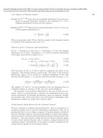
Below
is
an
example
of
a
dataset
designed
for
linear
regression.
The
input
variable
is
generated
randomly
and
the
target
variable
is
generated
as
a
linear
combination
of
that
input
variable
plus
an
error
term.


import
numpy
as
np

import
matplotlib.pyplot
as
plt

import
seaborn
as
sns



#
generate
data

np.random.seed(123)

N
=
20


beta0
=
-4

beta1
=
2

x
=
np.random.randn(N)

e
=
np.random.randn(N)

y
=
beta0
+
beta1*x
+
e

true_x
=
np.linspace(min(x),
max(x),
100)

true_y
=
beta0
+
beta1*true_x



#
plot

fig,
ax
=
plt.subplots()

sns.scatterplot(x,
y,
s
=
40,
label
=
'Data')

sns.lineplot(true_x,
true_y,
color
=
'red',
label
=
'True
Model')

ax.set_xlabel('x',
fontsize
=
14)

ax.set_title(fr"$y
=
{beta0}
+
${beta1}$x
+
\epsilon$",
fontsize
=
16)

ax.set_ylabel('y',
fontsize=14,
rotation=0,
labelpad=10)

ax.legend(loc
=
4)

sns.despine()


../../_images/concept_2_0.png

Parameter
Estimation
The
previous
section
covers
the
entire
structure
we
assume
our
data
follows
in
linear
regression.
The
machine
learning
task
is
then
to
estimate
the
parameters
in
 .
These
estimates
are
represented
by

estimates
give
us
fitted
values
for
our
target
variable,
represented
by


̂ 

̂ 
0

,…,

̂ 


or
 ̂ .
The

.

This
task
can
be
accomplished
in
two
ways
which,
though
slightly
different
conceptually,
are
identical
mathematically.
The
first
approach
is
through
the
lens
of
minimizing
loss.
A
common
practice
in
machine
learning
is
to
choose
a
loss
function
that
defines
how
well
a
model
with
a
given
set
of
parameter
estimates
the
observed
data.
The
most
common
loss
function
for
linear
regression
is
squared
error
loss.
This
says
the
loss
of
our
model
is
proportional
to
the
sum
of
squared
differences
between
the
true



values
and
the
fitted
values,


̂ 

.
We
then
fit
the
model
by
finding
the

estimates
 
that
minimize
this
loss
function.
This
approach
is
covered
in
the
subsection
Approach
1:
Minimizing
Loss.
̂ 

The
second
approach
is
through
the
lens
of
maximizing
likelihood.
Another
common
practice
in
machine
learning
is
to
model
the
target
as
a
random
variable
whose
distribution
depends
on
one
or
more
parameters,
and
then
find
the
parameters
that
maximize
its
likelihood.
Under
this
approach,
we
will
represent
the
target
with

treating
it
as
a
random
variable.
The
most
common
model
for

mean


(

) =

⊤


since
we
are


in
linear
regression
is
a
Normal
random
variable
with

.
That
is,
we
assume
|

∼ (

⊤

,

2

),

and
we
find
the
values
of
 ̂ 
to
maximize
the
likelihood.
This
approach
is
covered
in
subsection
Approach
2:
Maximizing
Likelihood.
Once
we’ve
estimated
 ,
our
model
is
fit
and
we
can
make
predictions.
The
below
graph
is
the
same
as
the
one
above
but
includes
our
estimated
line-of-best-fit,
obtained
by
calculating


̂ 
0


and


̂ 
1

.


#
generate
data

np.random.seed(123)

N
=
20

beta0
=
-4

beta1
=
2

x
=
np.random.randn(N)

e
=
np.random.randn(N)

y
=
beta0
+
beta1*x
+
e

true_x
=
np.linspace(min(x),
max(x),
100)

true_y
=
beta0
+
beta1*true_x



#
estimate
model


beta1_hat
=
sum((x
-
np.mean(x))*(y
-
np.mean(y)))/sum((x
-
np.mean(x))**2)

beta0_hat
=
np.mean(y)
-
beta1_hat*np.mean(x)

fit_y
=
beta0_hat
+
beta1_hat*true_x



#
plot

fig,
ax
=
plt.subplots()

sns.scatterplot(x,
y,
s
=
40,
label
=
'Data')

sns.lineplot(true_x,
true_y,
color
=
'red',
label
=
'True
Model')

sns.lineplot(true_x,
fit_y,
color
=
'purple',
label
=
'Estimated
Model')

ax.set_xlabel('x',
fontsize
=
14)


ax.set_title(fr"Linear
Regression
for
$y
=
{beta0}
+
${beta1}$x
+
\epsilon$",
fontsize

=
16)

ax.set_ylabel('y',
fontsize=14,
rotation=0,
labelpad=10)

ax.legend(loc
=
4)

sns.despine()


../../_images/concept_4_0.png

Extensions
of
Ordinary
Linear
Regression
There
are
many
important
extensions
to
linear
regression
which
make
the
model
more
flexible.
Those
include
Regularized
Regression—which
balances
the
bias-variance
tradeoff
for
high-dimensional
regression
models—
Bayesian
Regression—which
allows
for
prior
distributions
on
the
coefficients—and
GLMs—which
introduce
nonlinearity
to
regression
models.
These
extensions
are
discussed
in
the
next
chapter.

Approach
1:
Minimizing
Loss

1.
Simple
Linear
Regression
Model
Structure

Simple
linear
regression
models
the
target
variable,
 ,
as
a
linear
function
of
just
one
predictor
variable,
 ,
plus
an
error
term,
 .
We
can
write
the
entire
model
for
the

=

+

0

th


observation
as
+

1

Fitting
the
model
then
consists
of
estimating
two
parameters:

parameters

given


̂ 
0


and


̂ 
1

.

0


and


1

.
We
call
our
estimates
of
these

,
respectively.
Once
we’ve
made
these
estimates,
we
can
form
our
prediction
for
any


with
̂ 

̂  =

0

̂ 

+

1

.

One
way
to
find
these
estimates
is
by
minimizing
a
loss
function.
Typically,
this
loss
function
is
the
residual
sum

of
squares
(RSS).
The
RSS
is
calculated
with

(

̂ 
0

,

̂ 
1

1
) =

2 ∑

(

−

̂ 

2

) .

=1

We
divide
the
sum
of
squared
errors
by
2
in
order
to
simplify
the
math,
as
shown
below.
Note
that
doing
this
does
not
affect
our
estimates
because
it
does
not
affect
which


̂ 
0


and


̂ 
1


minimize
the
RSS.

Parameter
Estimation
Having
chosen
a
loss
function,
we
are
ready
to
derive
our
estimates.
First,
let’s
rewrite
the
RSS
in
terms
of
the
estimates:

(

̂ 
0

,

̂ 
1

1
) =

2 ∑
=1

(

− (

̂ 
0

+

̂ 
1

2

)) .


To
find
the
intercept
estimate,
start
by
taking
the
derivative
of
the
RSS
with
respect
to

̂ 

∂(

0

∂

̂ 

,

)

1

= −

̂ 

∑

0

=1

= −

̂ 

−

(

̂ 

(¯ −

0

0

̂ 

−

̂ 

−

1

̂ 

This
gives
our
intercept
estimate,


¯ ),
̂ 
0

:

̂  ¯
.

= ¯ −

1

,
in
terms
of
the
slope
estimate,


̂ 
0

:

)

1

where
 ¯ 
and
 ¯ 
are
the
sample
means.
Then
set
that
derivative
equal
to
0
and
solve
for


0

̂ 
0

.
To
find
the
slope
estimate,
again
start

̂ 
1

by
taking
the
derivative
of
the
RSS:
∂(
∂

̂ 
0

̂ 

,

1

)
= −

̂ 

∑

1

=1

Setting
this
equal
to
0
and
substituting
for


∑

(

̂ 
0

̂ 

−

0

.

)

1

,
we
get

̂ 

− (¯ −

̂ 

−

(

1

̂ 

¯) −

= 0

)

1

=1

̂ 
1

∑

− ¯)

(

=

∑

=1

− ¯)

(

=1

∑

̂ 

=

1

∑

=1

(

− ¯)

(

− ¯)

.

=1

To
put
this
in
a
more
standard
form,
we
use
a
slight
algebra
trick.
Note
that

− ¯) = 0

(

∑
=1

for
any
constant
 
and
any
collection


1,


with
sample
mean
 ¯ 
(this
can
easily
be
verified
by
expanding

…,

the
sum).
Since
 ¯ 
is
a
constant,
we
can
then
subtract
∑
∑

=1

¯(

− ¯)

=1


from
the
numerator
and


¯(

− ¯)


from
the
denominator
without
affecting
our
slope
estimate.
Finally,
we
get
∑

̂ 

=

1

=1

(

− ¯ )(

− ¯)
.

∑

=1

(

− ¯)

2

2.
Multiple
Regression
Model
Structure
In
multiple
regression,
we
assume
our
target
variable
to
be
a
linear
combination
of
multiple
predictor
variables.
Letting



be
the


th


predictor
for
observation
 ,
we
can
write
the
model
as
=

Using
the
vectors


0

+

1

1

+ ⋯ +

+

.


and
 
defined
in
the
previous
section,
this
can
be
written
more
compactly
as
=

⊤

+

.

Then
define
 ̂ 
the
same
way
as
 
except
replace
the
parameters
with
their
estimates.
We
again
want
to
find
the
vector
 ̂ 
that
minimizes
the
RSS:

(

̂ 
) =

1

2

⊤

(
2 ∑

−

̂ 

)

1
=

=1

2 ∑

(

−

2

̂  ) ,

=1

Minimizing
this
loss
function
is
easier
when
working
with
matrices
rather
than
sums.
Define
 
and
 
with
⎡
=

⎢
⎢
⎣

which
gives


̂  =

̂ 

∈ ℝ

1

…

⎡

⎤
⎥
⎥

∈ ℝ

⊤
1

⎤

⎢
⎥
= ⎢ … ⎥ ∈ ℝ
⎢
⎥

,

⎦

⎣

⊤

×(

+1)

,

⎦

.
Then,
we
can
equivalently
write
the
loss
function
as
(

̂ 
) =

1
(
2

−

̂  ⊤
) (

−

̂ 
).


Parameter
Estimation
We
can
estimate
the
parameters
in
the
same
way
as
we
did
for
simple
linear
regression,
only
this
time
calculating
the
derivative
of
the
RSS
with
respect
to
the
entire
parameter
vector.
First,
note
the
commonlyused
matrix
derivative
below
[1].
 Math
Note
For
a
symmetric
matrix


,
∂
(

−

)

⊤

(

−

) = −2

⊤

(

−

)

∂

Applying
the
result
of
the
Math
Note,
we
get
the
derivative
of
the
RSS
with
respect
to
 ̂ 
(note
that
the
identity
matrix
takes
the
place
of


):
1

̂ 
) =

(

(

̂  ⊤
) (

−

̂ 
)

−

2
̂ 
)

∂(

⊤

= −

(

̂ 
).

−

̂ 

∂

We
get
our
parameter
estimates
by
setting
this
derivative
equal
to
0
and
solving
for
 ̂ :
(

⊤

)
 

̂ 
̂ 

⊤

=
= (

⊤

)

⊤

⊤

A
helpful
guide
for
matrix
calculus
is
The
Matrix
Cookbook

[1]

Approach
2:
Maximizing
Likelihood

1.
Simple
Linear
Regression
Model
Structure
Using
the
maximum
likelihood
approach,
we
set
up
the
regression
model
probabilistically.
Since
we
are
treating
the
target
as
a
random
variable,
we
will
capitalize
it.
As
before,
we
assume
=

only
now
we
give


the


0

+

+

1


a
distribution
(we
don’t
do
the
same
for


,


since
its
value
is
known).
Typically,
we
assume


are
independently
Normally
distributed
with
mean
0
and
an
unknown
variance.
That
is,
i.i.d.

∼

2

 (0,

).

The
assumption
that
the
variance
is
identical
across
observations
is
called
homoskedasticity.
This
is
required
for
the
following
derivations,
though
there
are
heteroskedasticity-robust
estimates
that
do
not
make
this
assumption.

Since


0


and


1


are
fixed
parameters
and



is
known,
the
only
source
of
randomness
in

i.i.d.

∼

(

0

+

1

,

2


is


.
Therefore,

),

since
a
Normal
random
variable
plus
a
constant
is
another
Normal
random
variable
with
a
shifted
mean.
Parameter
Estimation
The
task
of
fitting
the
linear
regression
model
then
consists
of
estimating
the
parameters
with
maximum
likelihood.
The
joint
likelihood
and
log-likelihood
across
observations
are
as
follows.


(

0,

1;

1,

…,

) =

(

∏

0,

1;

)

=1

1
=

∏

(

2‾‾
√‾

=1

(
∝ exp

−

− (

exp −
(

− (

0

+

))

1

(

0,

1;

1,

…,

) = −

Our


̂ 
0


and


̂ 
1

(

∑

2

2

− (

2

+

0

2

)

1
log

2

)

2

2

=1

))

1

2

2

∑

(

+

0

1

)) .

=1


estimates
are
the
values
that
maximize
the
log-likelihood
given
above.
Notice
that
this
is

equivalent
to
finding
the


̂ 
0


and


̂ 
1


that
minimize
the
RSS,
our
loss
function
from
the
previous
section:
1
RSS =

2 ∑

̂ 

− (

(

2

̂ 

+

0

)) .

1

=1

In
other
words,
we
are
solving
the
same
optimization
problem
we
did
in
the
last
section.
Since
it’s
the
same
problem,
it
has
the
same
solution!
(This
can
also
of
course
be
checked
by
differentiating
and
optimizing
for

and


̂ 
0

).
Therefore,
as
with
the
loss
minimization
approach,
the
parameter
estimates
from
the
likelihood
1
̂ 

maximization
approach
are
̂ 
0

̂ 
1

=

̂  ¯

¯ −
∑

1

=1

=

(

− ¯ )(

¯)

−

.

∑

=1

2
− ¯)

(

2.
Multiple
Regression
Still
assuming
Normally-distributed
errors
but
adding
more
than
one
predictor,
we
have
i.i.d.

∼

(

⊤

2

,

).

We
can
then
solve
the
same
maximum
likelihood
problem.
Calculating
the
log-likelihood
as
we
did
above
for
simple
linear
regression,
we
have

log

(

0,

1;

1,

…,

1

) = −

∑

2

2

(

−

2

⊤

)

=1

1
= −
2

2

(

̂  ⊤
) (

−

−

̂ 
).

Again,
maximizing
this
quantity
is
the
same
as
minimizing
the
RSS,
as
we
did
under
the
loss
minimization
approach.
We
therefore
obtain
the
same
solution:
̂ 

= (

⊤

)

−1

⊤

.

Construction
This
section
demonstrates
how
to
construct
a
linear
regression
model
using
only
numpy.
To
do
this,
we
generate
a
class
named
LinearRegression.
We
use
this
class
to
train
the
model
and
make
future
predictions.
The
first
method
in
the
LinearRegression
class
is
fit(),
which
takes
care
of
estimating
the
 
parameters.
This
simply
consists
of
calculating
̂ 

= (

The
fit
method
also
makes
in-sample
predictions
with


(

̂ 
) =

⊤

−1

)

⊤


and
calculates
the
training
loss
with

̂ 

̂  =

1
2 ∑

(

−

̂ 

2

) .

=1

The
second
method
is
predict(),
which
forms
out-of-sample
predictions.
Given
a
test
set
of
predictors

fitted
values
with


′

̂  =

′

.

̂ 

′

,
we
can
form


import
numpy
as
np


import
matplotlib.pyplot
as
plt

import
seaborn
as
sns


class
LinearRegression:







def
fit(self,
X,
y,
intercept
=
False):











#
record
data
and
dimensions









if
intercept
==
False:
#
add
intercept
(if
not
already
included)














ones
=
np.ones(len(X)).reshape(len(X),
1)
#
column
of
ones














X
=
np.concatenate((ones,
X),
axis
=
1)









self.X
=
np.array(X)









self.y
=
np.array(y)









self.N,
self.D
=
self.X.shape



















#
estimate
parameters









XtX
=
np.dot(self.X.T,
self.X)









XtX_inverse
=
np.linalg.inv(XtX)









Xty
=
np.dot(self.X.T,
self.y)









self.beta_hats
=
np.dot(XtX_inverse,
Xty)



















#
make
in-sample
predictions









self.y_hat
=
np.dot(self.X,
self.beta_hats)



















#
calculate
loss









self.L
=
.5*np.sum((self.y
-
self.y_hat)**2)















def
predict(self,
X_test,
intercept
=
True):



















#
form
predictions









self.y_test_hat
=
np.dot(X_test,
self.beta_hats)


Let’s
try
out
our
LinearRegression
class
with
some
data.
Here
we
use
the
Boston
housing
dataset
from
sklearn.datasets.
The
target
variable
in
this
dataset
is
median
neighborhood
home
value.
The
predictors
are
all

continuous
and
represent
factors
possibly
related
to
the
median
home
value,
such
as
average
rooms
per
house.
Hit
“Click
to
show”
to
see
the
code
that
loads
this
data.
from
sklearn
import
datasets

boston
=
datasets.load_boston()


X
=
boston['data']

y
=
boston['target']


With
the
class
built
and
the
data
loaded,
we
are
ready
to
run
our
regression
model.
This
is
as
simple
as
instantiating
the
model
and
applying
fit(),
as
shown
below.
model
=
LinearRegression()
#
instantiate
model

model.fit(X,
y,
intercept
=
False)
#
fit
model


Let’s
then
see
how
well
our
fitted
values
model
the
true
target
values.
The
closer
the
points
lie
to
the
45-degree
line,
the
more
accurate
the
fit.
The
model
seems
to
do
reasonably
well;
our
predictions
definitely
follow
the
true
values
quite
well,
although
we
would
like
the
fit
to
be
a
bit
tighter.
 Note
Note
the
handful
of
observations
with



exactly.
This
is
due
to
censorship
in
the
data
collection

= 50

process.
It
appears
neighborhoods
with
average
home
values
above
$50,000
were
assigned
a
value
of
50
even.

fig,
ax
=
plt.subplots()

sns.scatterplot(model.y,
model.y_hat)

ax.set_xlabel(r'$y$',
size
=
16)

ax.set_ylabel(r'$\hat{y}$',
rotation
=
0,
size
=
16,
labelpad
=
15)

ax.set_title(r'$y$
vs.
$\hat{y}$',
size
=
20,
pad
=
10)

sns.despine()


../../_images/construction_10_0.png

Implementation


This
section
demonstrates
how
to
fit
a
regression
model
in
Python
in
practice.
The
two
most
common
packages
for
fitting
regression
models
in
Python
are
scikit-learn
and
statsmodels.
Both
methods
are
shown
before.
First,
let’s
import
the
data
and
necessary
packages.
We’ll
again
be
using
the
Boston
housing
dataset
from
sklearn.datasets.
import
matplotlib.pyplot
as
plt

import
seaborn
as
sns

from
sklearn
import
datasets

boston
=
datasets.load_boston()

X_train
=
boston['data']

y_train
=
boston['target']


Scikit-Learn
Fitting
the
model
in
scikit-learn
is
very
similar
to
how
we
fit
our
model
from
scratch
in
the
previous
section.
The
model
is
fit
in
two
steps:
first
instantiate
the
model
and
second
use
the
fit()
method
to
train
it.
from
sklearn.linear_model
import
LinearRegression

sklearn_model
=
LinearRegression()

sklearn_model.fit(X_train,
y_train);


As
before,
we
can
plot
our
fitted
values
against
the
true
values.
To
form
predictions
with
the
scikit-learn
model,
we
can
use
the
predict
method.
Reassuringly,
we
get
the
same
plot
as
before.
sklearn_predictions
=
sklearn_model.predict(X_train)

fig,
ax
=
plt.subplots()

sns.scatterplot(y_train,
sklearn_predictions)

ax.set_xlabel(r'$y$',
size
=
16)

ax.set_ylabel(r'$\hat{y}$',
rotation
=
0,
size
=
16,
labelpad
=
15)

ax.set_title(r'$y$
vs.
$\hat{y}$',
size
=
20,
pad
=
10)

sns.despine()


../../_images/code_7_0.png
We
can
also
check
the
estimated
parameters
using
the
coef_
attribute
as
follows
(note
that
only
the
first
few
are
printed).
predictors
=
boston.feature_names

beta_hats
=
sklearn_model.coef_

print('\n'.join([f'{predictors[i]}:
{round(beta_hats[i],
3)}'
for
i
in
range(3)]))


CRIM:
-0.108

ZN:
0.046

INDUS:
0.021


Statsmodels
statsmodels
is
another
package
frequently
used
for
running
linear
regression
in
Python.
There
are
two
ways
to
run

regression
in
statsmodels.
The
first
uses
numpy
arrays
like
we
did
in
the
previous
section.
An
example
is
given
below.
 Note
Note
two
subtle
differences
between
this
model
and
the
models
we’ve
previously
built.
First,
we
have
to
manually
add
a
constant
to
the
predictor
dataframe
in
order
to
give
our
model
an
intercept
term.
Second,
we
supply
the
training
data
when
instantiating
the
model,
rather
than
when
fitting
it.

import
statsmodels.api
as
sm



X_train_with_constant
=
sm.add_constant(X_train)

sm_model1
=
sm.OLS(y_train,
X_train_with_constant)

sm_fit1
=
sm_model1.fit()

sm_predictions1
=
sm_fit1.predict(X_train_with_constant)


The
second
way
to
run
regression
in
statsmodels
is
with
R-style
formulas
and
pandas
dataframes.
This
allows
us
to
identify
predictors
and
target
variables
by
name.
An
example
is
given
below.

import
pandas
as
pd

df
=
pd.DataFrame(X_train,
columns
=
boston['feature_names'])

df['target']
=
y_train

display(df.head())



formula
=
'target
~
'
+
'
+
'.join(boston['feature_names'])

print('formula:',
formula)


CRIM

ZN

INDUS

CHAS

NOX

RM

AGE

DIS

RAD

TAX

PTRATIO

0

0.00632

18.0

2.31

0.0

0.538

6.575

65.2

4.0900

1.0

296.0

15.3

396.9

1

0.02731

0.0

7.07

0.0

0.469

6.421

78.9

4.9671

2.0

242.0

17.8

396.9

2

0.02729

0.0

7.07

0.0

0.469

7.185

61.1

4.9671

2.0

242.0

17.8

392.8

3

0.03237

0.0

2.18

0.0

0.458

6.998

45.8

6.0622

3.0

222.0

18.7

394.6

4

0.06905

0.0

2.18

0.0

0.458

7.147

54.2

6.0622

3.0

222.0

18.7

396.9

formula:
target
~
CRIM
+
ZN
+
INDUS
+
CHAS
+
NOX
+
RM
+
AGE
+
DIS
+
RAD
+
TAX
+

PTRATIO
+
B
+
LSTAT


import
statsmodels.formula.api
as
smf



sm_model2
=
smf.ols(formula,
data
=
df)

sm_fit2
=
sm_model2.fit()

sm_predictions2
=
sm_fit2.predict(df)


Concept
Linear
regression
can
be
extended
in
a
number
of
ways
to
fit
various
modeling
needs.
Regularized
regression
penalizes
the
magnitude
of
the
regression
coefficients
to
avoid
overfitting,
which
is
particularly
helpful
for
models
using
a
large
number
of
predictors.
Bayesian
regression
places
a
prior
distribution
on
the
regression
coefficients
in
order
to
reconcile
existing
beliefs
about
these
parameters
with
information
gained
from
new
data.
Finally,
generalized
linear
models
(GLMs)
expand
on
ordinary
linear
regression
by
changing
the
assumed
error
structure
and
allowing
for
the
expected
value
of
the
target
variable
to
be
a
nonlinear
function
of
the
predictors.
These
extensions
are
described,
derived,
and
demonstrated
in
detail
this
chapter.

Regularized
Regression

Regression
models,
especially
those
fit
to
high-dimensional
data,
may
be
prone
to
overfitting.
One
way
to
ameliorate
this
issue
is
by
penalizing
the
magnitude
of
the
 ̂ 
coefficient
estimates.
This
has
the
effect
of
shrinking
these
estimates
toward
0,
which
ideally
prevents
the
model
from
capturing
spurious
relationships
between
weak
predictors
and
the
target
variable.
This
section
reviews
the
two
most
common
methods
for
regularized
regression:
Ridge
and
Lasso.

Ridge
Regression
Like
ordinary
linear
regression,
Ridge
regression
estimates
the
coefficients
by
minimizing
a
loss
function
on
the
training
data.
Unlike
ordinary
linear
regression,
the
loss
function
for
Ridge
regression
penalizes
large
values
of
the


estimates.
Specifically,
Ridge
regression
minimizes
the
sum
of
the
RSS
and
the
L2
norm
of
 ̂ :

̂ 

Ridge (

̂ 
) =

1
2

(

−

̂ 

)

⊤

(

−

2

̂ 

) +

̂ 

2 ∑

.

=1

Here,
 
is
a
tuning
parameter
which
represents
the
amount
of
regularization.
A
large
 
means
a
greater
penalty
on
the
 ̂ 
estimates,
meaning
more
shrinkage
of
these
estimates
toward
0.
 
is
not
estimated
by
the
model
but
rather
chosen
before
fitting,
typically
through
cross
validation.
 Note
Note
that
the
Ridge
loss
function
does
not
penalize
the
magnitude
of
the
intercept
estimate,

Intuitively,
a
greater
intercept
does
not
suggest
overfitting.

̂ 
0

.


As
in
ordinary
linear
regression,
we
start
estimating
 ̂ 
by
taking
the
derivative
of
the
loss
function.
First
note
that
since


̂ 
0


is
not
penalized,
⎡
∂

2

̂ 

̂ ( 2 ∑

∂

=
)

=1

⎢

where


′


is
the
identity
matrix
of
size


+ 1

⎥

1

⎥

...

⎥

̂ 

⎣

⎦
 ̂
,

′

=

⎥

̂ 

⎢
⎢

⎤

0

⎢


except
the
first
element
is
a
0.
Then,
adding
in
the
derivative
of
the

RSS
discussed
in
chapter
1,
we
get
̂ 
)

∂Ridge (

= −
∂

⊤

(

̂ 

̂ 

−

) +

̂ 
.

′

Setting
this
equal
to
0
and
solving
for
 ̂ ,
we
get
our
estimates:
̂ 
(

⊤

+

′

⊤

) =
̂ 

= (

⊤

+

−1

′

⊤

,

)

Lasso
Regression
Lasso
regression
differs
from
Ridge
regression
in
that
its
loss
function
uses
the
L1
norm
for
the
 ̂ 
estimates
rather
than
the
L2
norm.
This
means
we
penalize
the
sum
of
absolute
values
of
the
 ̂ s,
rather
than
the
sum
of
their
squares.

̂ 
) =

Lasso (

1
2

(

̂ 

−

⊤

)

−

(

̂ 

) +

∑

|

|.

=1

As
usual,
let’s
then
calculate
the
gradient
of
the
loss
function
with
respect
to
 ̂ :
̂ 
)

∂(

= −
∂

where
again
we
use


′

̂ 

⊤

(

−

̂ 

)

+

′

 sign(

̂ 
),


rather
than
 
since
the
magnitude
of
the
intercept
estimate


̂ 
0


is
not
penalized.

Unfortunately,
we
cannot
find
a
closed-form
solution
for
the
 ̂ 
that
minimize
the
Lasso
loss.
Numerous
methods
exist
for
estimating
the
 ̂ ,
though
using
the
gradient
calculated
above
we
could
easily
reach
an
estimate
through
gradient
descent.
The
construction
in
the
next
section
uses
this
approach.

Bayesian
Regression

In
the
Bayesian
approach
to
statistical
inference,
we
treat
our
parameters
as
random
variables
and
assign
them
a
prior
distribution.
This
forces
our
estimates
to
reconcile
our
existing
beliefs
about
these
parameters
with
new
information
given
by
the
data.
This
approach
can
be
applied
to
linear
regression
by
assigning
the
regression
coefficients
a
prior
distribution.
We
also
may
wish
to
perform
Bayesian
regression
not
because
of
a
prior
belief
about
the
coefficients
but
in
order
to
minimize
model
complexity.
By
assigning
the
parameters
a
prior
distribution
with
mean
0,
we
force
the
posterior
estimates
to
be
closer
to
0
than
they
would
otherwise.
This
is
a
form
of
regularization
similar
to
the
Ridge
and
Lasso
methods
discussed
in
the
previous
section.

The
Bayesian
Structure
To
demonstrate
Bayesian
regression,
we’ll
follow
three
typical
steps
to
Bayesian
analysis:
writing
the
likelihood,
writing
the
prior
density,
and
using
Bayes’
Rule
to
get
the
posterior
density.
In
the
results
below,
we
use
the
posterior
density
to
calculate
the
maximum-a-posteriori
(MAP)—the
equivalent
of
calculating
the
 ̂ 
estimates
in
ordinary
linear
regression.

1.
The
Likelihood


As
in
the
typical
regression
set-up,
let’s
assume
i.i.d.

∼

⊤

 (

2

,

).

We
can
write
the
collection
of
observations
jointly
as
∼  (

where


∈ ℝ


and


=

2

×

∈ ℝ

,

),


for
some
known
scalar


2

.
Note
that
 
is
a
vector
of
random
variables

—it
is
not
capitalized
in
order
to
distinguish
it
from
a
matrix.
 Note
See
this
lecture
for
an
example
of
Bayesian
regression
without
the
assumption
of
known
variance.

We
can
then
get
our
likelihood
and
log-likelihood
using
the
Multivariate
Normal.
1
(

;

,

1

) =

exp

−

(

‾‾‾‾‾‾‾
(2
) | ‾
|
√‾
1
∝ exp

−

(

(

−

(

;

,

) = −

−

)

⊤

⊤

−1

(

−

(

−

)

⊤

−1

−1

(

−

)

)

)

)

2

1
log

)

(
2

(

−

).

2

2.
The
Prior
Now,
let’s
assign
 
a
prior
distribution.
We
typically
assume
∼  (0,

where


∈ ℝ


and


=


for
some
scalar
 .
We
choose
 
(and
therefore
 )
ourselves,
with
a

×

∈ ℝ

),

greater
 
giving
less
weight
to
the
prior.
The
prior
density
is
given
by
1
(

1

) =

exp

1
∝ exp
1
log

(

⊤

−

(

−1

)

2

−1

)

2
⊤

) = −

⊤

−

(

‾‾‾‾‾‾‾
(2
) | ‾
|
√‾

−1

.

2

3.
The
Posterior
We
are
then
interested
in
a
posterior
density
of
 
given
the
data,
 
and
 .
Bayes’
rule
tells
us
that
the
posterior
density
of
the
coefficients
is
proportional
to
the
likelihood
of
the
data
times
the
prior
density
of
the
coefficients.
Using
the
two
previous
results,
we
have

log

(

|

,

) ∝

(

|

,

) = log

(

;

,
(

) (
;

,

)
) + log

1
= −

(

−

)

⊤

−1

(

) +
1

(

−

) −

2
1
= −
2

⊤

−1

+

2

2

(

−

)

⊤

1
(

−

) −

⊤

+

2

where
 
is
some
constant
that
we
don’t
care
about.

Results
Intuition
Often
in
the
Bayesian
setting
it
is
infeasible
to
obtain
the
entire
posterior
distribution.
Instead,
one
typically
looks
at
the
maximum-a-posteriori
(MAP),
the
value
of
the
parameters
that
maximize
the
posterior
density.
In
our
case,
the
MAP
is
the
 ̂ 
that
maximizes


log

̂ 
|

(

1
,

) = −

2

2

(

̂  ⊤
) (

−

1

̂ 
) −

−

⊤

̂ 

This
is
equivalent
to
finding
the
 ̂ 
that
minimizes
the
following
loss
function,
where

(

̂ 
) =

1
(

̂  ⊤
) (

−

⊤

̂ 
) +

−

2

̂ 

= 1/

.

̂ 

2

1
=

̂ 
.

2

(

̂  ⊤
) (

−

̂ 
) +

−

2

̂ 
2 ∑

.

=0

Notice
that
this
is
extremely
close
to
the
Ridge
loss
function
discussed
in
the
previous
section—it
is
not
quite
equal
to
the
Ridge
loss
function
since
it
also
penalizes
the
magnitude
of
the
intercept,
though
this
difference
could
be
eliminated
by
changing
the
prior
distribution
of
the
intercept.
This
shows
that
Bayesian
regression
with
a
mean-zero
Normal
prior
distribution
is
essentially
equivalent
to
Ridge
regression.
Decreasing
 ,
just
like
increasing
 ,
increases
the
amount
of
regularization.

Full
Results
Now
let’s
actually
derive
the
MAP
by
calculating
the
gradient
of
the
log
posterior
density.
 Math
Note
For
a
symmetric
matrix


,
∂
(

−

)

⊤

(

−

⊤

) = −2

(

−

)

∂

This
implies
that
∂

∂

⊤

=

∂

(0 −

)

⊤

(0 −

) = 2

.

∂

Using
the
Math
Note
above,
we
have
log

(

̂ 
|

1
,

) = −

(

−

)

⊤

−1

1
(

−

) −

2
∂
log

(

|

,

) =

⊤

−1

2

⊤

−1

(

−

) −

−1

.

∂

We
calculate
the
MAP
by
setting
this
gradient
equal
to
0:
̂ 

= (

⊤

−1

1
=

(

+

−1

−1

−1

1

⊤

+

2

⊤

−1

)

)

1
2

⊤

.

GLMs

Ordinary
linear
regression
comes
with
several
assumptions
that
can
be
relaxed
with
a
more
flexible
model
class:
generalized
linear
models
(GLMs).
Specifically,
OLS
assumes
1.
The
target
variable
is
a
linear
function
of
the
input
variables
2.
The
errors
are
Normally
distributed
3.
The
variance
of
the
errors
is
constant
When
these
assumptions
are
violated,
GLMs
might
be
the
answer.

GLM
Structure
A
GLM
consists
of
a
link
function
and
a
random
component.
The
random
component
identifies
the
distribution
of
the
target
variable



conditional
on
the
input
variables


variable
where
the
rate
parameter



depends
on


.

.
For
instance,
we
might
model



as
a
Poisson
random


The
link
function
specifies
how



relates
to
the
expected
value
of
the
target
variable,


function
of
the
input
variables,
i.e.


⊤

=

=

(

)

.
Let
 
be
a
linear


for
some
coefficients
 .
We
then
chose
a
nonlinear
link
function
to

relate
 
to
 .
For
link
function
 
we
have
=

(

).

In
a
GLM,
we
calculate
 
before
calculating
 ,
so
we
often
work
with
the
inverse
of
 :
=

−1

(

)

 Note
Note
that
because



is
a
function
of
the
data,
it
will
vary
for
each
observation
(though
the
 s
will

not).

In
total
then,
a
GLM
assumes
∼
=
=

where
 
is
some
distribution
with
mean
parameter


−1

(

⊤

)
,

.

Fitting
a
GLM
“Fitting”
a
GLM,
like
fitting
ordinary
linear
regression,
really
consists
of
estimating
the
coefficients,
 .
Once
we
know
 ,
we
have
 .
Once
we
have
a
link
function,
 
gives
us
 
through

1.
Specify
the
distribution
of

2.
Specify
the
link
function


,
indexed
by
its
mean
parameter

=

−1

.
A
GLM
can
be
fit
in
these
four
steps:

.

.

(

)

3.
Identify
a
loss
function.
This
is
typically
the
negative
log-likelihood.
4.
Find
the
 ̂ 
that
minimize
that
loss
function.
In
general,
we
can
write
the
log-likelihood
across
our
observations
for
a
GLM
as
follows.

log

({

}

=1

;{

}

=1 )

=

∑

log

(

;

) =

=1

∑

log

−1

(

(

);

) =

∑

=1

log

(

−1

(

⊤

);

).

=1

This
shows
how
the
log-likelihood
depends
on
 ,
the
parameters
we
want
to
estimate.
To
fit
the
GLM,
we
want
to
find
the
 ̂ 
to
maximize
this
log-likelihood.

Example:
Poisson
Regression
Step
1
Suppose
we
choose
to
model



conditional
on



as
a
Poisson
random
variable
with
rate
parameter

|

∼ Pois(

:

).

Since
the
expected
value
of
a
Poisson
random
variable
is
its
rate
parameter,


(

) =

=

.

Step
2
To
determine
the
link
function,
let’s
think
in
terms
of
its
inverse,

negative
and


=

−1

(

)

.
We
know
that



could
be
anywhere
in
the
reals
since
it
is
a
linear
function
of

= exp(

),

meaning
=

(

) = log(

).

This
is
the
“canonical
link”
function
for
Poisson
regression.
More
on
that
here.
Step
3
Let’s
derive
the
negative
log-likelihood
for
the
Poisson.
Let


= [

⊤
1,

…,


must
be
non-

.
One
function
that
works
is

]

.

 Math
Note
The
PMF
for


∼ Pois(

)


is
−

( ) =

−

∝

.

!

(

;{

}

=1

) =

∏

exp(−

)

=1

log

(

;{

}

=1

) =

log

∑

−

.

=1

Now
let’s
get
our
loss
function,
the
negative
log-likelihood.
Recall
that
this
should
be
in
terms
of
 
rather
than

since
 
is
what
we
control.



(

) = −

log(exp(

∑
(

)) − exp(

)
)

=1

=

∑

(exp(

) −

)

=1

=

∑

⊤

(exp(

⊤

) −

).

=1

Step
4
We
obtain
 ̂ 
by
minimizing
this
loss
function.
Let’s
take
the
derivative
of
the
loss
function
with
respect
to
 .
∂

(

)
=

∑

∂

⊤

(exp(

)

−

).

=1

Ideally,
we
would
solve
for
 ̂ 
by
setting
this
gradient
equal
to
0.
Unfortunately,
there
is
no
closed-form
solution.
Instead,
we
can
approximate
 ̂ 
through
gradient
descent.
This
is
done
in
the
construction
section.
Since
gradient
descent
calculates
this
gradient
a
large
number
of
times,
it’s
important
to
calculate
it
efficiently.
Let’s
see
if
we
can
clean
this
expression
up.
First
recall
that
$

̂ 

̂  =

⊤

= exp(

̂ 

$

).

The
loss
function
can
then
be
written
as
∂

(

̂ 
)
=

∂

̂ 

∑

(

̂ 

−

).

=1

Further,
this
can
be
written
in
matrix
form
as

∂

(

̂ 
)
=

∂

⊤

( ̂ −

),

̂ 

where
 ̂ 
is
the
vector
of
fitted
values.
Finally
note
that
this
vector
can
be
calculated
as
̂  = exp(

̂ 
),

where
the
exponential
function
is
applied
element-wise
to
each
observation.

Many
other
GLMs
exist.
One
important
example
is
logistic
regression,
the
topic
of
the
next
chapter.

Construction
This
pages
in
this
section
construct
classes
to
run
the
linear
regression
extensions
discussed
in
the
previous
section.
The

first
builds
a
Ridge
and
Lasso
regression
model,
the
second
builds
a
Bayesian
regression
model,
and
the
third
builds
a
Poisson
regression
model.

Regularized
Regression


import
numpy
as
np


import
matplotlib.pyplot
as
plt

import
seaborn
as
sns

from
sklearn
import
datasets



boston
=
datasets.load_boston()

X
=
boston['data']

y
=
boston['target']


Before
building
the
RegularizedRegression
class,
let’s
define
a
few
helper
functions.
The
first
function
standardizes
the
data
by
removing
the
mean
and
dividing
by
the
standard
deviation.
This
is
the
equivalent
of
the
StandardScaler
from
scikit-learn.
The
sign
function
simply
returns
the
sign
of
each
element
in
an
array.
This
is
useful
for
calculating
the
gradient
in
Lasso
regression.
The
first_element_zero
option
makes
the
function
return
a
0
(rather
than
a
-1
or
1)
for
the
first
element.
As
discussed
in
the
concept
section,
this
prevents
Lasso
regression
from
penalizing
the
magnitude
of
the
intercept.
def
standard_scaler(X):





means
=
X.mean(0)





stds
=
X.std(0)





return
(X
-
means)/stds



def
sign(x,
first_element_zero
=
False):





signs
=
(-1)**(x
<
0)





if
first_element_zero:










signs[0]
=
0





return
signs


The
RegularizedRegression
class
below
contains
methods
for
fitting
Ridge
and
Lasso
regression.
The
first
method,
record_info,
handles
standardization,
adds
an
intercept
to
the
predictors,
and
records
the
necessary
values.
The

second,
fit_ridge,
fits
Ridge
regression
using
̂ 

= (

⊤

+

′

−1

)

⊤

.

The
third
method,
fit_lasso,
estimates
the
regression
parameters
using
gradient
descent.
The
gradient
is
the
derivative
of
the
Lasso
loss
function:
∂

̂ 

)

(

= −
∂

̂ 

⊤

(

−

̂ 

) +

′

 sign(

̂ 
).

The
gradient
descent
used
here
simply
adjusts
the
parameters
a
fixed
number
of
times
(determined
by
n_iters).
There
many
more
efficient
ways
to
implement
gradient
descent,
though
we
use
a
simple
implementation
here
to
keep
focus
on
Lasso
regression.

class
RegularizedRegression:















def
_record_info(self,
X,
y,
lam,
intercept,
standardize):



















#
standardize










if
standardize
==
True:














X
=
standard_scaler(X)



















#
add
intercept









if
intercept
==
False:














ones
=
np.ones(len(X)).reshape(len(X),
1)
#
column
of
ones














X
=
np.concatenate((ones,
X),
axis
=
1)
#
concatenate























#
record
values









self.X
=
np.array(X)









self.y
=
np.array(y)









self.N,
self.D
=
self.X.shape









self.lam
=
lam















def
fit_ridge(self,
X,
y,
lam
=
0,
intercept
=
False,
standardize
=
True):



















#
record
data
and
dimensions









self._record_info(X,
y,
lam,
intercept,
standardize)



















#
estimate
parameters









XtX
=
np.dot(self.X.T,
self.X)









I_prime
=
np.eye(self.D)









I_prime[0,0]
=
0










XtX_plus_lam_inverse
=
np.linalg.inv(XtX
+
self.lam*I_prime)










Xty
=
np.dot(self.X.T,
self.y)









self.beta_hats
=
np.dot(XtX_plus_lam_inverse,
Xty)



















#
get
fitted
values









self.y_hat
=
np.dot(self.X,
self.beta_hats)

























def
fit_lasso(self,
X,
y,
lam
=
0,
n_iters
=
2000,



















lr
=
0.0001,
intercept
=
False,
standardize
=
True):











#
record
data
and
dimensions









self._record_info(X,
y,
lam,
intercept,
standardize)



















#
estimate
parameters









beta_hats
=
np.random.randn(self.D)









for
i
in
range(n_iters):













dL_dbeta
=
-self.X.T
@
(self.y
-
(self.X
@
beta_hats))
+

self.lam*sign(beta_hats,
True)













beta_hats
-=
lr*dL_dbeta










self.beta_hats
=
beta_hats



















#
get
fitted
values









self.y_hat
=
np.dot(self.X,
self.beta_hats)


The
following
cell
runs
Ridge
and
Lasso
regression
for
the
Boston
housing
dataset.
For
simplicity,
we
somewhat
arbitrarily
choose


= 10

—in
practice,
this
value
should
be
chosen
through
cross
validation.

#
set
lambda

lam
=
10



#
fit
ridge

ridge_model
=
RegularizedRegression()

ridge_model.fit_ridge(X,
y,
lam)



#
fit
lasso

lasso_model
=
RegularizedRegression()

lasso_model.fit_lasso(X,
y,
lam)


The
below
graphic
shows
the
coefficient
estimates
using
Ridge
and
Lasso
regression
with
a
changing
value
of
 .
Note
that



is
identical
to
ordinary
linear
regression.
As
expected,
the
magnitude
of
the
coefficient
estimates

= 0

decreases
as
 
increases.


Xs
=
['X'+str(i
+
1)
for
i
in
range(X.shape[1])]

lams
=
[10**4,
10**2,
0]



fig,
ax
=
plt.subplots(nrows
=
2,
ncols
=
len(lams),
figsize
=
(6*len(lams),
10),

sharey
=
True)

for
i,
lam
in
enumerate(lams):











ridge_model
=
RegularizedRegression()






ridge_model.fit_lasso(X,
y,
lam)






ridge_betas
=
ridge_model.beta_hats[1:]





sns.barplot(Xs,
ridge_betas,
ax
=
ax[0,
i],
palette
=
'PuBu')





ax[0,
i].set(xlabel
=
'Regressor',
title
=
fr'Ridge
Coefficients
with
$\lambda
=
$

{lam}')





ax[0,
i].set(xticks
=
np.arange(0,
len(Xs),
2),
xticklabels
=
Xs[::2])











lasso_model
=
RegularizedRegression()





lasso_model.fit_lasso(X,
y,
lam)






lasso_betas
=
lasso_model.beta_hats[1:]





sns.barplot(Xs,
lasso_betas,
ax
=
ax[1,
i],
palette
=
'PuBu')





ax[1,
i].set(xlabel
=
'Regressor',
title
=
fr'Lasso
Coefficients
with
$\lambda
=
$

{lam}')





ax[1,
i].set(xticks
=
np.arange(0,
len(Xs),
2),
xticklabels
=
Xs[::2])



ax[0,0].set(ylabel
=
'Coefficient')

ax[1,0].set(ylabel
=
'Coefficient')

plt.subplots_adjust(wspace
=
0.2,
hspace
=
0.4)

sns.despine()

sns.set_context('talk');


../../_images/regularized_9_0.png

Bayesian
Regression
import
numpy
as
np


import
matplotlib.pyplot
as
plt

import
seaborn
as
sns

from
sklearn
import
datasets

boston
=
datasets.load_boston()

X
=
boston['data']


y
=
boston['target']


The
BayesianRegression
class
estimates
the
regression
coefficients
using
1

(

Note
that
this
assumes


2

⊤

2

−1

1
+

)

1

⊤

2

.


and
 
are
known.
We
can
determine
the
influence
of
the
prior
distribution
by

manipulationg
 ,
though
there
are
principled
ways
to
choose
 .
There
are
also
principled
Bayesian
methods
to
model

2


(see
here),
though
for
simplicity
we
will
estimate
it
with
the
typical
OLS
estimate:
2

̂  =

,
− (

where


+ 1)


is
the
sum
of
squared
errors
from
an
ordinary
linear
regression,



is
the
number
of
observations,
and


is
the
number
of
predictors.
Using
the
linear
regression
model
from
chapter
1,
this
comes
out
to
about
11.8.
class
BayesianRegression:











def
fit(self,
X,
y,
sigma_squared,
tau,
add_intercept
=
True):



















#
record
info









if
add_intercept:













ones
=
np.ones(len(X)).reshape((len(X),1))













X
=
np.append(ones,
np.array(X),
axis
=
1)










self.X
=
X









self.y
=
y



















#
fit









XtX
=
np.dot(X.T,
X)/sigma_squared









I
=
np.eye(X.shape[1])/tau









inverse
=
np.linalg.inv(XtX
+
I)









Xty
=
np.dot(X.T,
y)/sigma_squared









self.beta_hats
=
np.dot(inverse
,
Xty)



















#
fitted
values









self.y_hat
=
np.dot(X,
self.beta_hats)























Let’s
fit
a
Bayesian
regression
model
on
the
Boston
housing
dataset.
We’ll
use


2

= 11.8


and


= 10

.

sigma_squared
=
11.8

tau
=
10


model
=
BayesianRegression()

model.fit(X,
y,
sigma_squared,
tau)


The
below
plot
shows
the
estimated
coefficients
for
varying
levels
of
 .
A
lower
value
of
 
indicates
a
stronger
prior,
and
therefore
a
greater
pull
of
the
coefficients
towards
their
expected
value
(in
this
case,
0).
As
expected,
the
estimates
approach
0
as
 
decreases.
Xs
=
['X'+str(i
+
1)
for
i
in
range(X.shape[1])]

taus
=
[100,
10,
1]



fig,
ax
=
plt.subplots(ncols
=
len(taus),
figsize
=
(20,
4.5),
sharey
=
True)

for
i,
tau
in
enumerate(taus):





model
=
BayesianRegression()





model.fit(X,
y,
sigma_squared,
tau)






betas
=
model.beta_hats[1:]





sns.barplot(Xs,
betas,
ax
=
ax[i],
palette
=
'PuBu')





ax[i].set(xlabel
=
'Regressor',
title
=
fr'Regression
Coefficients
with
$\tau
=
$

{tau}')





ax[i].set(xticks
=
np.arange(0,
len(Xs),
2),
xticklabels
=
Xs[::2])



ax[0].set(ylabel
=
'Coefficient')

sns.set_context("talk")

sns.despine();


../../_images/bayesian_7_0.png

GLMs
import
numpy
as
np


import
matplotlib.pyplot
as
plt

import
seaborn
as
sns

from
sklearn
import
datasets


boston
=
datasets.load_boston()

X
=
boston['data']

y
=
boston['target']


In
this
section,
we’ll
build
a
class
for
fitting
Poisson
regression
models.
First,
let’s
again
create
the
standard_scaler
function
to
standardize
our
input
data.
def
standard_scaler(X):





means
=
X.mean(0)





stds
=
X.std(0)





return
(X
-
means)/stds


We
saw
in
the
GLM
concept
page
that
the
gradient
of
the
loss
function
(the
negative
log-likelihood)
in
a
Poisson
model
is
given
by
̂ 
)

∂(

=
∂

⊤

( ̂ −

),

̂ 

where

̂  = exp(

̂ 
).

The
class
below
constructs
Poisson
regression
using
gradient
descent
with
these
results.
Again,
for
simplicity
we
use
a
straightforward
implementation
of
gradient
descent
with
a
fixed
number
of
iterations
and
a
constant
learning
rate.


class
PoissonRegression:











def
fit(self,
X,
y,
n_iter
=
1000,
lr
=
0.00001,
add_intercept
=
True,
standardize

=
True):



















#
record
stuff









if
standardize:













X
=
standard_scaler(X)









if
add_intercept:













ones
=
np.ones(len(X)).reshape((len(X),
1))













X
=
np.append(ones,
X,
axis
=
1)









self.X
=
X









self.y
=
y



















#
get
coefficients









beta_hats
=
np.zeros(X.shape[1])









for
i
in
range(n_iter):













y_hat
=
np.exp(np.dot(X,
beta_hats))













dLdbeta
=
np.dot(X.T,
y_hat
-
y)













beta_hats
-=
lr*dLdbeta












#
save
coefficients
and
fitted
values









self.beta_hats
=
beta_hats









self.y_hat
=
y_hat
















Now
we
can
fit
the
model
on
the
Boston
housing
dataset,
as
below.
model
=
PoissonRegression()

model.fit(X,
y)


The
plot
below
shows
the
observed
versus
fitted
values
for
our
target
variable.
It
is
worth
noting
that
there
does
not
appear
to
be
a
pattern
of
under-estimating
for
high
target
values
like
we
saw
in
the
ordinary
linear
regression
example.
In
other
words,
we
do
not
see
a
pattern
in
the
residuals,
suggesting
Poisson
regression
might
be
a
more
fitting
method
for
this
problem.
fig,
ax
=
plt.subplots()

sns.scatterplot(model.y,
model.y_hat)

ax.set_xlabel(r'$y$',
size
=
16)

ax.set_ylabel(r'$\hat{y}$',
rotation
=
0,
size
=
16,
labelpad
=
15)

ax.set_title(r'$y$
vs.
$\hat{y}$',
size
=
20,
pad
=
10)

sns.despine()


../../_images/GLMs_9_0.png

Implementation
This
section
shows
how
the
linear
regression
extensions
discussed
in
this
chapter
are
typically
fit
in
Python.
First
let’s
import
the
Boston
housing
dataset.
import
numpy
as
np


import
matplotlib.pyplot
as
plt

import
seaborn
as
sns

from
sklearn
import
datasets

boston
=
datasets.load_boston()


X_train
=
boston['data']

y_train
=
boston['target']


Regularized
Regression
Both
Ridge
and
Lasso
regression
can
be
easily
fit
using
scikit-learn.
A
bare-bones
implementation
is
provided
below.
Note
that
the
regularization
parameter
alpha
(which
we
called
 )
is
chosen
arbitrarily.


from
sklearn.linear_model
import
Ridge,
Lasso

alpha
=
1



#
Ridge

ridge_model
=
Ridge(alpha
=
alpha)

ridge_model.fit(X_train,
y_train)





#
Lasso

lasso_model
=
Lasso(alpha
=
alpha)

lasso_model.fit(X_train,
y_train);


In
practice,
however,
we
want
to
choose
alpha
through
cross
validation.
This
is
easily
implemented
in
scikit-learn
by
designating
a
set
of
alpha
values
to
try
and
fitting
the
model
with
RidgeCV
or
LassoCV.
from
sklearn.linear_model
import
RidgeCV,
LassoCV

alphas
=
[0.01,
1,
100]



#
Ridge

ridgeCV_model
=
RidgeCV(alphas
=
alphas)

ridgeCV_model.fit(X_train,
y_train)



#
Lasso


lassoCV_model
=
LassoCV(alphas
=
alphas)

lassoCV_model.fit(X_train,
y_train);


We
can
then
see
which
values
of
alpha
performed
best
with
the
following.
print('Ridge
alpha:',
ridgeCV.alpha_)

print('Lasso
alpha:',
lassoCV.alpha_)


Ridge
alpha:
0.01

Lasso
alpha:
1.0


Bayesian
Regression
We
can
also
fit
Bayesian
regression
using
scikit-learn
(though
another
popular
package
is
pymc3).
A
very
straightforward
implementation
is
provided
below.
from
sklearn.linear_model
import
BayesianRidge

bayes_model
=
BayesianRidge()

bayes_model.fit(X_train,
y_train);


This
is
not,
however,
identical
to
our
construction
in
the
previous
section
since
it
infers
the


2


and
 
parameters,

rather
than
taking
those
as
fixed
inputs.
More
information
can
be
found
here.
The
hidden
chunk
below
demonstrates
a
hacky
solution
for
running
Bayesian
regression
in
scikit-learn
using
known
values
for


2


and
 ,
though
it
is
hard

to
imagine
a
practical
reason
to
do
so
By
default,
Bayesian
regression
in
scikit-learn
treats


=

1
2


and


=

1


as
random
variables
and
assigns

them
the
following
prior
distributions

Note
that


(

) =

1


and


(

) =

2

1

.
To
fix


∼ Gamma(

1,

2)

∼ Gamma(

1,

2 ).

2


and
 ,
we
can
provide
an
extremely
strong
prior
on
 
and
 ,

2

guaranteeing
that
their
estimates
will
be
approximately
equal
to
their
expected
value.
Suppose
we
want
to
use


2

= 11.8


and


= 10

,
or
equivalently


=

1
11.8

,


=

1
10

.
Then
let

1

This
guarantees
that


2

1

= 10000 ⋅

2

= 10000,

1

= 10000 ⋅

2

= 10000.

,
11.8

1

,

10


and
 
will
be
approximately
equal
to
their
pre-determined
values.
This
can
be

implemented
in
scikit-learn
as
follows


big_number
=
10**5




#
alpha

alpha
=
1/11.8

alpha_1
=
big_number*alpha

alpha_2
=
big_number



#
lambda


lam
=
1/10

lambda_1
=
big_number*lam

lambda_2
=
big_number



#
fit


bayes_model
=
BayesianRidge(alpha_1
=
alpha_1,
alpha_2
=
alpha_2,
alpha_init
=
alpha,






















lambda_1
=
lambda_1,
lambda_2
=
lambda_2,
lambda_init
=
lam)

bayes_model.fit(X_train,
y_train);


Poisson
Regression
GLMs
are
most
commonly
fit
in
Python
through
the
GLM
class
from
statsmodels.
A
simple
Poisson
regression
example
is
given
below.
As
we
saw
in
the
GLM
concept
section,
a
GLM
is
comprised
of
a
random
distribution
and
a
link
function.
We
identify
the
random
distribution
through
the
family
argument
to
GLM
(e.g.
below,
we
specify
the
Poisson
family).
The
default
link
function
depends
on
the
random
distribution.
By
default,
the
Poisson
model
uses
the
link
function
=

(

) = log(

),

which
is
what
we
use
below.
For
more
information
on
the
possible
distributions
and
link
functions,
check
out
the
statsmodels
GLM
docs.
import
statsmodels.api
as
sm

X_train_with_constant
=
sm.add_constant(X_train)



poisson_model
=
sm.GLM(y_train,
X_train,
family=sm.families.Poisson())

poisson_model.fit();


Concept
A
classifier
is
a
supervised
learning
algorithm
that
attempts
to
identify
an
observation’s
membership
in
one
of
two
or
more
groups.
In
other
words,
the
target
variable
in
classification
represents
a
class
from
a
finite
set
rather
than
a
continuous
number.
Examples
include
detecting
spam
emails
or
identifying
hand-written
digits.
This
chapter
and
the
next
cover
discriminative
and
generative
classification,
respectively.
Discriminative
classification
directly
models
an
observation’s
class
membership
as
a
function
of
its
input
variables.
Generative
classification
instead
views
the
input
variables
as
a
function
of
the
observation’s
class.
It
first
models
the
prior
probability
that
an
observation
belongs
to
a
given
class,
then
calculates
the
probability
of
observing
the
observation’s
input
variables
conditional
on
its
class,
and
finally
solves
for
the
posterior
probability
of
belonging
to
a
given
class
using
Bayes’
Rule.
More
on
that
in
the
following
chapter.
The
most
common
method
in
this
chapter
by
far
is
logistic
regression.
This
is
not,
however,
the
only
discriminative
classifier.
This
chapter
also
introduces
two
others:
the
Perceptron
Algorithm
and
Fisher’s
Linear
Discriminant.

Logistic
Regression

In
linear
regression,
we
modeled
our
target
variable
as
a
linear
combination
of
the
predictors
plus
a
random
error
term.
This
meant
that
the
fitted
value
could
be
any
real
number.
Since
our
target
in
classification
is
not
any
real
number,
the
same
approach
wouldn’t
make
sense
in
this
context.
Instead,
logistic
regression
models
a
function
of
the
target
variable
as
a
linear
combination
of
the
predictors,
then
converts
this
function
into
a
fitted
value
in
the
desired
range.

Binary
Logistic
Regression

Model
Structure


In
the
binary
case,
we
denote
our
target
variable
with

probability
that


∈ {0, 1}


is
in
class
1.
We
want
a
way
to
express


and
1.
Consider
the
following
function,
called
the
log-odds
of

(

.
Let


=

(

= 1)


be
our
estimate
of
the


as
a
function
of
the
predictors
(

)
that
is
between
0

.

) = log

.

(1 −

)

Note
that
its
domain
is
(0, 1) 
and
its
range
is
all
real
numbers.
This
suggests
that
modeling
the
log-odds
as
a
linear
combination
of
the
predictors—resulting
in


(

) ∈ ℝ

—would
correspond
to
modeling



as
a
value

between
0
and
1.
This
is
exactly
what
logistic
regression
does.
Specifically,
it
assumes
the
following
structure.
̂ 
( ̂  ) = log
( 1 −

̂ 

=

̂  )

̂ 

+

0

1

1

̂ 

+ ⋯ +

⊤

̂ 

=

.

 Math
Note
The
logistic
function
is
a
common
function
in
statistics
and
machine
learning.
The
logistic
function
of
 ,
written
as


,
is
given
by

( )

1

( ) =

.
1 + exp(− )

The
derivative
of
the
logistic
function
is
quite
nice.
′

0 + exp(− )
(1 + exp(− ))

Ultimately,
we
are
interested
in

is
the
logistic
function
of


⊤

̂ 

̂ 

exp(− )

1

( ) =

=

2

⋅

=

1 + exp(− )

,
not
the
log-odds


( ̂  )

( )(1 −

( )).

1 + exp(− )

.
Rearranging
the
log-odds
expression,
we
find
that


̂ 


(see
the
Math
Note
above
for
information
on
the
logistic
function).
That
is,
1

⊤

̂  =

̂ 

(

) =

.

⊤

1 + exp(−

̂ 

)

By
the
derivative
of
the
logistic
function,
this
also
implies
that
⊤

∂ ̂ 

∂

̂ 

(

)

⊤

=
∂

=

̂ 

∂

⊤

̂ 

(

)

̂ 

1 −
(

(

̂ 

)
⋅
)

Parameter
Estimation
We
will
estimate
 ̂ 
with
maximum
likelihood.
The
PMF
for


(

) =

(1 −

)

1−

=

Notice
that
this
gives
us
the
correct
probability
for


(

= 0

∼ Bern(

⊤

)


and


(1 −

= 1


is
given
by

)

⊤

(

1−

))

.

.

Now
assume
we
observe
the
target
variables
for
our
training
data,
meaning


1,

…,


crystalize
into


1,

We
can
write
the
likelihood
and
log-likelihood.

(

;{

,

}

=1

) =

∏

(

)

=1

=

∏

(

⊤

)

(1 −

(

⊤

))

1−

=1

log

(

;{

,

}

=1

) =

∑

log

(

⊤

) + (1 −

) log(1 −

(

⊤

))

=1

Next,
we
want
to
find
the
values
of
 ̂ 
that
maximize
this
log-likelihood.
Using
the
derivative
of
the
logistic
function
for


⊤


discussed
above,
we
get

…,

.


∂ log

(

;{

,

}

=1

)

1
=

∂

∑

(

=1

=

∂

)

1
− (1 −

)

∂

)

(1 −

∑

⊤

(

⋅

⊤

⊤

(

1 −

)) ⋅

− (1 −

)

⊤

(

(

∂
⊤

⊤

(

)

⋅
)

∂

) ⋅

=1

=

−

∑

⊤

(

)

=1

=

∑

(

−

)

.

=1

Next,
let


= (

⊤
1

2

…

)

be
the
vector
of
probabilities.
Then
we
can
write
this
derivative
in
matrix

form
as
∂ log

(

;{

,

}

=1

)
=

(

−

).

∂

Ideally,
we
would
find
 ̂ 
by
setting
this
gradient
equal
to
0
and
solving
for
 .
Unfortunately,
there
is
no
closed
form
solution.
Instead,
we
can
estimate
 ̂ 
through
gradient
descent
using
the
derivative
above.
Note
that
gradient
descent
minimizes
a
loss
function,
rather
than
maximizing
a
likelihood
function.
To
get
a
loss
function,
we
would
simply
take
the
negative
log-likelihood.
Alternatively,
we
could
do
gradient
ascent
on
the
loglikelihood.

Multiclass
Logistic
Regression
Multiclass
logistic
regression
generalizes
the
binary
case
into
the
case
where
there
are
three
or
more
possible
classes.

Notation
First,
let’s
establish
some
notation.
Suppose
there
are
 
classes
total.
When



can
fall
into
three
or
more

classes,
it
is
best
to
write
it
as
a
one-hot
vector:
a
vector
of
all
zeros
and
a
single
one,
with
the
location
of
the
one
indicating
the
variable’s
value.
For
instance,

=

⎡ 0 ⎤
⎢
⎥
⎢ 1 ⎥
⎢
⎢

...

⎥

∈ ℝ

⎥

⎣ 0 ⎦

indicates
that
the


th


observation
belongs
to
the
second
of
 
classes.
Similarly,
let


probabilities
for
observation
 ,
where
the


th

̂ 


be
a
vector
of
estimated


entry
indicates
the
probability
that
observation
 
belongs
to
class


.
Note
that
this
vector
must
be
non-negative
and
add
to
1.
For
the
example
above,
⎡ 0.01 ⎤
⎢
̂ 

=

⎥
⎢ 0.98 ⎥
⎢
⎢

...

⎥

∈ ℝ

⎥

⎣ 0.00 ⎦

would
be
a
pretty
good
estimate.
Finally,
we
need
to
write
the
coefficients
for
each
class.
Suppose
we
have
 
predictor
variables,
including
the
intercept
(i.e.


∈ ℝ


where
the
first
term
in



is
an
appended
1).
We
can
let


coefficient
estimates
for
class
 .
Alternatively,
we
can
use
the
matrix
̂ 

= [

̂ 
1

…

̂ 

] ∈ ℝ

to
jointly
represent
the
coefficients
of
all
classes.

Model
Structure
Let’s
start
by
defining


̂ 


as
̂  =

⊤

̂ 

∈ ℝ

.

×

,

̂ 


be
the
length- 
vector
of