Glassner DEEP LEARNING From Basics to Practice
Bạn đang xem bản rút gọn của tài liệu. Xem và tải ngay bản đầy đủ của tài liệu tại đây (17.71 MB, 104 trang )
Free Chapter!
DEEP LEARNING:
From Basics
to Practice
Andrew Glassner
www.glassner.com
@AndrewGlassner
Deep Learning:
From Basics to Practice
Copyright (c) 2018 by Andrew Glassner
www.glassner.com / @AndrewGlassner
All rights reserved. No part of this book, except as noted below, may be reproduced,
stored in a retrieval system, or transmitted in any form or by any means, without
the prior written permission of the author, except in the case of brief quotations
embedded in critical articles or reviews.
The above reservation of rights does not apply to the program files associated with
this book (available on GitHub), or to the images and figures (also available on
GitHub), which are released under the MIT license. Any images or figures that are
not original to the author retain their original copyrights and protections, as noted
in the book and on the web pages where the images are provided.
All software in this book, or in its associated repositories, is provided “as is,” without warranty of any kind, express or implied, including but not limited to the
warranties of merchantability, fitness for a particular pupose, and noninfringement. In no event shall the authors or copyright holders be liable for any claim,
damages or other liability, whether in an action of contract, tort, or otherwise,
arising from, out of or in connection with the software or the use or other dealings
in the software.
First published February 20, 2018
Version 1.0.1
March 3, 2018
Version 1.1
March 22, 2018
Published by The Imaginary Institute, Seattle, WA.
Contact:
Chapter 18
Backpropagation
This chapter is from my book, “Deep Learning: From Principles to
Practice,” by Andrew Glassner. I’m making it freely available! Feel free
to share this and other bonus chapters with friends and colleagues.
The book is in 2 volumes, available here:
/> />You can download all the figures in the entire book, and all the Python
notebooks, for free from my GitHub site:
/>To get a free Kindle reader for your device, visit
/>
Chapter 18: Backpropagation
Contents
18.1 Why This Chapter Is Here.............................. 706
18.1.1 A Word On Subtlety...................................... 708
18.2 A Very Slow Way to Learn............................. 709
18.2.1 A Slow Way to Learn.................................... 712
18.2.2 A Faster Way to Learn................................. 716
18.3 No Activation Functions for Now................ 718
18.4 Neuron Outputs and Network Error........... 719
18.4.1 Errors Change Proportionally..................... 720
18.5 A Tiny Neural Network.................................. 726
18.6 Step 1: Deltas for the Output Neurons....... 732
18.7 Step 2: Using Deltas to Change Weights..... 745
18.8 Step 3: Other Neuron Deltas........................ 750
18.9 Backprop in Action........................................ 758
18.10 Using Activation Functions......................... 765
18.11 The Learning Rate......................................... 774
18.11.1 Exploring the Learning Rate...................... 777
704
Chapter 18: Backpropagation
18.12 Discussion...................................................... 787
18.12.1 Backprop In One Place............................... 787
18.12.2 What Backprop Doesn’t Do...................... 789
18.12.3 What Backprop Does Do........................... 789
18.12.4 Keeping Neurons Happy........................... 790
18.12.5 Mini-Batches............................................... 795
18.12.6 Parallel Updates......................................... 796
18.12.7 Why Backprop Is Attractive...................... 797
18.12.8 Backprop Is Not Guaranteed ................... 797
18.12.9 A Little History........................................... 798
18.12.10 Digging into the Math.............................. 800
References............................................................... 802
705
Chapter 18: Backpropagation
18.1 Why This Chapter Is Here
This chapter is about training a neural network. The very basic idea is
appealingly simple. Suppose we’re training a categorizer, which will
tell us which of several given labels should be assigned to a given input.
It might tell us what animal is featured in a photo, or whether a bone
in an image is broken or not, or what song a particular bit of audio
belongs to.
Training this neural network involves handing it a sample, and asking
it to predict that sample’s label. If the prediction matches the label
that we previously determined for it, we move on to the next sample.
If the prediction is wrong, we change the network to help it do better
next time.
Easily said, but not so easily done. This chapter is about how we
“change the network” so that it learns, or improves its ability to make
correct predictions. This approach works beautifully not just for classifiers, but for almost any kind of neural network.
Contrast a feed-forward network of neurons to the dedicated classifiers we saw in Chapter 13. Each of those dedicated algorithms had
a customized, built-in learning method that measured the incoming
data to provide the information that classifier needed to know.
But a neural network is just a giant collection of neurons, each doing its
own little calculation and then passing on its results to other neurons.
Even when we organize them into layers, there’s no inherent learning
algorithm.
How can we train such a thing to produce the results we want? And
how can we do it efficiently?
706
Chapter 18: Backpropagation
The answer is called backpropagation, or simply backprop.
Without backprop, we wouldn’t have today’s widespread use of deep
learning, because we wouldn’t be able to train our models in reasonable amounts of time. With backprop, deep learning algorithms are
practical and plentiful.
Backprop is a low-level algorithm. When we use libraries to build and
train deep learning systems, their finely-tuned routines give us both
speed and accuracy. Except as an educational exercise, or to implement
some new idea, we’re likely to never write our own code to perform
backprop.
So why is this chapter here? Why should we bother knowing about this
low-level algorithm at all? There are at least four good reasons to have
a general knowledge of backpropagation.
First, it’s important to understand backprop because knowledge of
one’s tools is part of becoming a master in any field. Sailors at sea, and
pilots in the air, need to understand how their autopilots work in order
to use them properly. A photographer with an auto-focus camera
needs to know how that feature works, what its limits are, and how to
control it, so that she can work with the automated system to capture
the images she wants. A basic knowledge of the core techniques of any
field is part of the process of gaining proficiency and developing mastery. In this case, knowing something about backprop lets us read the
literature, talk to other people about deep learning ideas, and better
understand the algorithms and libraries we use.
Second, and more practically, knowing about backprop can help us
design networks that learn. When a network learns slowly, or not at
all, it can be because something is preventing backprop from running
properly. Backprop is a versatile and robust algorithm, but it’s not bulletproof. We can easily build networks where backprop won’t produce
useful changes, resulting in a network that stubbornly refuses to learn.
For those times when something’s going wrong with backprop, understanding the algorithm helps us fix things [Karpathy16].
707
Chapter 18: Backpropagation
Third, many important advances in neural networks rely on backprop
intimately. To learn these new ideas, and understand why they work
the way they do, it’s important to know the algorithms they’re building
on.
Finally, backprop is an elegant algorithm. It efficiently solves a problem that would otherwise require a prohibitive amount of time and
computer resources. It’s one of the conceptual treasures of the field.
As curious, thoughtful people it’s well worth our time to understand
this beautiful algorithm.
For these reasons and others, this chapter provides an introduction
to backprop. Generally speaking, introductions to backprop are presented mathematically, as a collection of equations with associated
discussion [Fullér10]. As usual, we’ll skip the mathematics and focus
instead on the concepts. The mechanics are common-sense at their
core, and don’t require any tools beyond basic arithmetic and the ideas
of a derivative and gradient, which we discussed in Chapter 5.
18.1.1 A Word On Subtlety
The backpropagation algorithm is not complicated. In fact, it’s remarkably simple, which is why it can be implemented so efficiently.
But simple does not always mean easy.
The backprop algorithm is subtle. In the discussion below, the algorithm will take shape through a process of observations and reasoning,
and these steps may take some thought. We’ll try to be clear about
every step, but making the leap from reading to understanding may
require some work.
It’s worth the effort.
708
Chapter 18: Backpropagation
18.2 A Very Slow Way to Learn
Let’s begin with a very slow way to train a neural network. This will
give us a good starting point, which we’ll then improve.
Suppose we’ve been given a brand-new neural network consisting of
hundreds or even tens of thousands of interconnected neurons. The
network was designed to classify each input into one of 5 categories.
So it has 5 outputs, which we’ll number 1 to 5, and whichever one has
the largest output is the network’s prediction for an input’s category.
Figure 18.1 shows the idea.
Figure 18.1: A neural network predicting the class of an input sample.
Starting at the bottom of Figure 18.1, we have a sample with four features and a label. The label tells us that the sample belongs to category
3. The features go into a neural network which has been designed to
provide 5 outputs, one for each class. In this example, the network has
incorrectly decided that the input belongs to class 1, because the largest output, 0.9, is from output number 1.
709
Chapter 18: Backpropagation
Consider the state of our brand-new network, before it has seen any
inputs. As we know from Chapter 16, each input to each neuron has
an associated weight. There could easily be hundreds of thousands,
or many millions, of weights in our network. Typically, all of these
weights will have been initialized with small random numbers.
Let’s now run one piece of labeled training data through the net, as
in Figure 18.1. The sample’s features go into the first layer of neurons,
and the outputs of those neurons go into more neurons, and so on,
until they finally arrive at the output neurons, when they become the
output of the network. The index of the output neuron with the largest
value is the predicted class for this sample.
Since we’re starting with random numbers for our weights, we’re likely
to get essentially random outputs. So there’s a 1 in 5 chance the network will happen to predict the right label for this sample. But there’s
a 4 in 5 chance it’ll get it wrong, so let’s assume that the network predicts the wrong category.
When the prediction doesn’t match the label, we can measure the error
numerically, coming up with a single number to tell us just how wrong
this answer is. We call this number the error score, or error, or
sometimes the loss (if the word “loss” seems like a strange synonym
for “error,” it may help to think to think of it as describing how much
information is “lost” if we categorize a sample using the output of the
classifier, rather than the label.).
The error (or loss) is a floating-point number that can take on any
value, though often we set things up so that it’s always positive. The
larger the error, the more “wrong” our network’s prediction is for the
label of this input.
An error of 0 means that the network predicted this sample’s label correctly. In a perfect world, we’d get the error down to 0 for every sample
in the training set. In practice, we usually settle for getting as close as
we can.
710
Chapter 18: Backpropagation
Let’s briefly recap some terminology from previous chapters. When we
speak of “the network’s error” with respect to a training set, we usually mean some kind of overall average that tells us how the network
is doing when taking all the training samples into consideration. We
call this the training error, since it’s the overall error we get from
predicting results from the training set. Similarly, the error from the
test or validation data is called the test error or validation error.
When the system is deployed, a measure of the mistakes it makes on
new data is called the generalization error, because it represents
how well (or poorly) the system manages to “generalize” from its training data to new, real-world data.
A nice way to think about the whole training process is to anthropomorphize the network. We can say that it “wants” to get its error down
to zero, and the whole point of the learning process is to help it achieve
that goal.
One advantage of this way of thinking is that we can make the network do anything we want, just by setting up the error to “punish” any
quality or behavior that we don’t want. Since the algorithms we’ll see
in this chapter are designed to minimize the error, we know that anything about the network’s behavior that contributes to the error will
get minimized.
The most natural thing to punish is getting the wrong answer, so the
error almost always includes a term that measures how far the output
is from the correct label. The worse the match between the prediction
and the label, the bigger this term will be. Since the network wants to
minimize the error, it will naturally minimize such mistakes.
This approach of “punishing” the network through the error score
means we can choose to include terms in the error for anything we can
measure and want to suppress. For example, another popular measure to add into the error is a regularization term, where we look
at the magnitude of all the weights in the network. As we’ll see later in
this chapter, we usually want those weights to be “small,” which often
means between −1 and 1. As the weights move beyond this range, we
711
Chapter 18: Backpropagation
add a larger number to the error. Since the network “wants” the smallest error possible, it will try to keep the weights small so that this term
remains small.
All of this raises the natural question of how on earth the network is
able to accomplish this goal of minimizing the error. That’s the point
of this chapter.
Let’s start with a basic error measure that only punishes a mismatch
between the network’s prediction and the label.
Our first algorithm for teaching the network will be just a thought
experiment, since it would be absurdly slow on today’s computers.
But the motivation is right, and this slow algorithm will form the conceptual basis for the more efficient techniques we’ll see later in this
chapter.
18.2.1 A Slow Way to Learn
Let’s stick with our running example of a classifier. We’ll give the network a sample and compare the system’s prediction with the sample’s
label.
If the network got it right and predicted the correct label, we won’t
change anything and we’ll move on to the next sample. As the wise
man said, “If it ain’t broke, don’t fix it” [Seung05].
But if the result for a particular sample is incorrect (that is, the category with the highest value does not match our label), we will try to
improve things. That is, we’ll learn from our mistakes.
How do we learn from this mistake? Let’s stick with this sample for
a while and try to help the network do a better job with it. First, we’ll
pick a small random number (which might be positive or negative).
Now we’ll pick one weight at random from the thousands or millions
of weights in the network, and we’ll add our small random value to
that weight.
712
Chapter 18: Backpropagation
Now we’ll evaluate our sample again. Everything up to that change will
be the same as before. But there will be a chain reaction of changes
in the outputs of the neurons starting at the weight we modified. The
new weight will produce a new input for the neuron that uses that
input, which will change that neuron’s output value, which will change
the output of every neuron that uses that output, which will change
the output of every neuron that uses any of those outputs, and so on.
Figure 18.2 shows this idea graphically.
Figure 18.2: Updating a single weight causes a chain reaction that ultimately can change the network’s outputs.
Figure 18.2 shows a network of 5 layers with 3 neurons each. Data
flows from the inputs at the left to the outputs at the right. For simplicity, not every neuron uses the output of every neuron on the previous
layer. In part (a) we select one weight at random, here shown in red
and marked w. In part (b) we modify the weight by adding a value m
to it, so the weight is now w+m. When we run the sample through the
network again, as shown in part (c), the new weight causes a change
713
Chapter 18: Backpropagation
in the output of the neuron it feeds into (in red). The output of that
neuron changes as a result, which causes the neurons it feeds into to
change their outputs, and the changes cascade all the way to the output layer.
Now that we have a new output, we can compare it to the label and
measure the new error. If the new error is less than the previous error,
then we’ve made things better! We’ll keep this change, and move on to
the next sample.
But if the results didn’t get better then we’ll undo this change, restoring the weight back to its previous value. We’ll then pick a new random
weight, change it by a newly-selected small random amount, and evaluate the network again.
We can continue this process of picking and nudging weights until the
results improve, or we decide we’ve tried enough times, or for any other
reason we decide to stop. Then we just move on to the next sample.
When we’ve used all the samples in our training set, we’ll just go
through them all again (maybe in a different order), over and over.
The idea is that we’ll improve a little bit from every mistake.
We can continue this process until the network classifies every input
correctly, or we’ve come close enough, or our patience is exhausted.
With this technique, we would expect the network to slowly improve,
though there may be setbacks along the way. For example, adjusting a
weight to improve one sample’s prediction might ruin the prediction
for one or more other samples. If so, when those samples come along
they will cause their own changes to improve their performance.
This thought algorithm isn’t perfect, because things could get stuck.
For example, there might be times when we need to adjust more than
one weight simultaneously. To fix that, we can imagine extending our
algorithm to assign multiple random changes to multiple random
weights. But let’s stick with the simpler version for now.
714
Chapter 18: Backpropagation
Given enough time and resources, the network would eventually find
a value for every weight that either predicts the right answer for every
sample, or it comes as close as that network possibly can.
The important word in that last sentence is eventually. As in, “The
water will boil, eventually,” or “The Andromeda galaxy will collide with
our Milky Way galaxy, eventually” [NASA12].
This technique, while a valid way to teach a network, is definitely not
practical. Modern networks can have millions of weights. Trying to
find the best values for all those weights with this algorithm is just not
realistic.
But this is the core idea. To train our network, we’ll watch its output,
and when it makes mistakes, we’ll adjust the weights to make those
mistakes less likely. Our goal in this chapter will be to take this rough
idea and re-structure it into a vastly more practical algorithm.
Before we move on, it’s worth noting that we’ve been talking about
weights, but not the bias term belonging to every neuron. We know
that every neuron’s bias gets added in along with the neuron’s weighted
inputs, so changing the bias would also change the output. Doesn’t that
mean that we want to adjust the bias values as well? We sure do. But
thanks to the bias trick we saw in Chapter 10, we don’t have to think
about the bias explicitly. That little bit of relabeling sets up the bias
to look like an input with its own weight, just like all the other inputs.
The beauty of this arrangement is that it means that as far as our training algorithm is concerned, the bias is just another weight to adjust. In
other words, all we need to think about is adjusting weights, and the
bias weights will automatically get adjusted along the way with all the
other weights.
Let’s now consider how we might improve our incredibly slow
weight-changing algorithm.
715
Chapter 18: Backpropagation
18.2.2 A Faster Way to Learn
The algorithm of the last section would improve our network, but at a
glacial pace.
One big source of inefficiency is that half of our adjustments to the
weights are in the wrong direction: we add a value when we should
instead have subtracted it, and vice-versa. That’s why we had to undo
our changes when the error went up. Another problem is that we tuned
each weight one by one, requiring us to evaluate an immense number
of samples. Let’s solve these problems.
We could avoid making mistakes if we knew beforehand whether we
wanted to nudge each weight along the number line to the right (that
is, make it more positive) or to the left (and make it more negative).
We can get exactly that information from the gradient of the error
with respect to that weight. Recall that we met the gradient in Chapter
5, where it told us how the height of a surface changes as each of its
parameters changes. Let’s narrow that down for the present case. In
1D (where the gradient is also called the derivative), the gradient is
the slope of a curve above a specific point. Our curve describes the network’s error, and our point is the value of a weight. If the slope of the
error (the gradient) above the weight is positive (that is, the line goes
up as we move to the right), then moving the point to the right will
cause the error to go up. More useful to us is that moving the point to
the left will cause the error to go down. If the slope of the error is negative, the situations are reversed.
Figure 18.3 shows two examples.
716
Chapter 18: Backpropagation
Figure 18.3: The gradient tells us what will happen to the error (the black
curves) if we move a weight to the right. The gradient is given by the
slope of the curve directly above the point we’re interested in. Lines that
go up as we move right have a positive slope, otherwise they are negative.
In Figure 18.3(a), we see that if we move the round weight to the right,
the error will increase, because the slope of the error is positive. To
reduce the error, we need to move the round point left. The square
point’s gradient is negative, so we reduce the error by moving that
point right. Part (b) shows the gradient for the round point is negative,
so moving to the right will reduce the error. The square point’s gradient is positive, so we reduce the error by moving that point to the left.
If we had the gradient for a weight, we could always adjust it exactly as
needed to make the error go down.
Using the gradients wouldn’t be much of an advantage if they were
time-consuming to compute, so as our second improvement let’s suppose that we can calculate the gradients for the weights very efficiently.
In fact, let’s suppose that we could quickly calculate the gradient for
every weight in the whole network. Then we could update all of the
weights simultaneously by adding a small value (positive or negative)
to each weight in the direction given by its own individual gradient.
That would be an immense time-saver.
717
Chapter 18: Backpropagation
Putting these together gives us a plan where we’ll run a sample through
the network, measure the output, compute the gradient for every
weight, and then use the gradient at each weight to move that weight
to the right or the left. This is exactly what we’re going to do.
This plan makes knowing the gradient an important issue. Finding the
gradient efficiently is the main goal of this chapter.
Before we continue, it’s worth noticing that this algorithm makes the
assumption that tweaking all the weights independently and simultaneously will lead to a reduction in the error. This is a bold assumption,
because we’ve already seen how changing one weight can cause ripple
effects through the rest of the network. Those effects could change the
values of other neurons, which in turn would change their gradients.
We won’t get into the details now, but we’ll see later that if we make
the changes to the weights small enough, that assumption will generally hold true, and the error will indeed go down.
18.3 No Activation Functions for
Now
For the next few sections in this chapter, we’re going to simplify the discussion by pretending that our neurons don’t have activation functions.
As we saw in Chapter 17, activation functions are essential to keep our
whole network from becoming nothing more than the equivalent of a
single neuron. So we need to use them.
But if we include them in our initial discussion of backprop, things
will get complicated, fast. If we leave activation functions out for just
a moment, the logic is much easier to follow. We’ll put them back in
again at the end.
718
Chapter 18: Backpropagation
Since we’re temporarily pretending that there are no activation functions in our neurons, neurons in the following discussions just sum
up their weighted inputs, and present that sum as their output, as in
Figure 18.4. As before, each weight is named with a two-letter composite of the neuron it’s coming from and the neuron it’s going into.
Figure 18.4: Neuron D simply sums up its incoming values, and presents
that sum as its output. Here we’ve explicit named the weights on each
connection into neuron D.
Until we put explicitly put activation functions back in, our neurons
will emit nothing more than the sum of their weighted inputs.
18.4 Neuron Outputs and Network
Error
Our goal is to reduce the overall error for a sample, by adjusting the
network’s weights.
We’ll do this in two steps. In the first step, we calculate and store a
number called the “delta” for every neuron. This number is related to
the network’s error, as we’ll see below. This step is performed by the
backpropagation algorithm.
719
Chapter 18: Backpropagation
The second step uses those delta values at the neurons to update the
weights. This step is called the update step. It’s not typically considered part of backpropagation, but sometimes people casually roll the
two steps together and call the whole thing “backpropagation.”
The overall plan now is to run a sample through the network, get the
prediction, and compare that prediction to the label to get an error. If
their error is greater than 0, we use it to compute and store a number
we’ll call “delta” at every neuron. We use these delta values and the
neuron outputs to calculate an update value for each weight. The final
step is to apply every weight’s individual update so that it takes on a
new value.
Then we move on to the next sample, and repeat the process, over and
over again until the predictions are all perfect or we decide to stop.
Let’s now look at this mysterious “delta” value that we store at each
neuron.
18.4.1 Errors Change Proportionally
There are two key observations that will make sense of everything to
follow. These are both based on how the network behaves when we
ignore the activation functions, which we’re doing for the moment. As
promised above, we’ll put them back in later in this chapter.
The first observation is this: When any neuron output in our network
changes, the output error changes by a proportional amount.
Let’s unpack that statement.
Since we’re ignoring activation functions, there are really only two
types of values we care about in the system: weights (which we can set
and change as we please), and neuron outputs (which are computed
automatically, and which are beyond our direct control). Except for
the very first layer, a neuron’s input values are each the output of a
720
Chapter 18: Backpropagation
previous neuron times the weight of the connection that output travels
on. Each neuron’s output is just the sum of all of these weighted inputs.
Figure 18.5 recaps this idea graphically.
Figure 18.5: A small neural network with 11 neurons organized in 4 layers.
Data flows from the inputs at the left to the outputs at the right. Each
neuron’s inputs come from the outputs of the neurons on the previous
layer. This type of diagram, though common, easily becomes dense and
confusing, even with color-coding. We will avoid it when possible.
We know that we’ll be changing weights to improve our network. But
sometimes it’s easier to think about looking at the change in a neuron’s
output. As long as we keep using the same input, the only reason a neuron’s output can change is because one of its weights has changed. So
in the rest of this chapter, any time we speak of the result of a change
in a neuron’s output, that came about because we changed one of the
weights that neuron depended on.
Let’s take this point of view now, and imagine we’re looking at a neuron whose output has just changed. What happens to the network’s
error as a result? Because the only operations that are being carried
out in our network are multiplication and addition, if we work through
the numbers we’ll see that the result of this change is that the change
in the error is proportional to the change in the neuron’s output.
721
Chapter 18: Backpropagation
In other words, to find the change in the error, we find the change in
the neuron’s output and multiply that by some particular value. If we
double the amount of change in the neuron’s output, we’ll double the
amount of change in the error. If we cut the neuron’s output change by
one-third, we’ll cut the change in the output by one-third.
The connection between any change in the neuron’s output and the
resulting change in the final error is just the neuron’s change times
some number. This number goes by various names, but the most popular is probably the lower-case Greek letter δ (delta), though sometimes
the upper-case version, Δ, is used. Mathematicians often use the delta
character to mean “change” of some sort, so this was a natural (if terse)
choice of name.
So every neuron has a “delta,” or δ, associated with it. This is a real
number that can be big or small, positive or negative. If the neuron’s
output changes by a particular amount (that is, it goes up or down),
we multiply that change by that neuron’s delta, and that tells us how
the entire network’s output will change.
Let’s draw a couple of pictures to show the “before” and “after” conditions of a neuron whose output changes. We’ll change the output of
the neuron using brute force: we’ll add some arbitrary number to the
summed inputs just before that value emerges as the neuron’s output.
As in Figure 18.2, we’ll use the letter m (for “modification”) for this
extra value.
Figure 18.6 shows the idea graphically.
722
Chapter 18: Backpropagation
Figure 18.6: Computing the change in the error due to a change in a
neuron’s output. Here we’re forcing a change in the neuron’s output by
adding an arbitrary amount m to the sum of the inputs. Because the
output will change by m, we know the change in the error is this difference m times the value of δ belonging to this neuron.
In Figure 18.6 we placed the value m inside the neuron. But we can
also change the output by changing one of the inputs. Let’s change the
value that’s coming in from neuron B. We know that the output of B
will get multiplied by the weight BD before it’s used by neuron D. So
let’s add our value m right after that weight has been applied. This will
have the same result as before, since we’re just adding m to the overall
sum that emerges from D. Figure 18.7 shows the idea. We can find the
change in the output like before, multiplying this change m in the output by δ.
723
Chapter 18: Backpropagation
Figure 18.7: A variation of Figure 18.6, where we add m to the output of B
(after it has been multiplied by the weight BD). The output of D is again
changed by m, and the change in the error is again m times this neuron’s
value of δ.
To recap, if we know the change in a neuron’s output, and we know the
value of delta for that neuron, then we can predict the change in the
error by multiplying that change in the output by that neuron’s delta.
This is a remarkable observation, because it shows us explicitly how
the error changes based on the change in output of each neuron. The
value of delta acts like an amplifier, making any change in the neuron’s
output have a bigger or smaller effect on the network’s error.
An interesting result of multiplying the neuron’s change in output with
its delta is that if the change in the output and the value of delta both
have the same sign (that is, both are positive or negative), then the
change in the error will be positive, meaning that the error will increase.
If the change in the output and delta have opposite signs (that is, one
724
Chapter 18: Backpropagation
is negative and one is positive), then the change in the error will be
negative, meaning that the error will decrease. That’s the case we want,
since our goal is always to make the error as small as possible.
For instance, suppose that neuron A has a delta of 2, and for some
reason its output changes by −2 (say, changing from 5 to 3). Since the
delta is positive and the change in output is negative, the change in
the error will also be negative. In numbers, 2×−2=−4, so the error will
drop by 4.
On the other hand, suppose the delta of A is −2, and its output changes
by +2 (say from 3 to 5). Again, the signs are different, so the error will
change by −2×2=−4, and again the error will reduce by 4.
But if the change in A’s output is −2, and the delta is also −2, then the
signs are the same. Since −2×−2=4, the error will increase by 4.
At the start of this section we said there were two key observations we
wanted to note. The first, as we’ve been discussing, is that if a neuron’s
output changes, the error changes by a proportional amount.
The second key observation is: this whole discussion applies just as
well to the weights. After all, the weights and the outputs are multiplied together. When we multiply two arbitrary numbers, such as a
and b, then we make the result bigger by adding something to either
the value of a or b. In terms of our network, we can say that when any
weight in our network changes, the error changes by a proportional
amount.
If we wanted, we could work out a delta for every weight. And that
would be perfect. We would know just how to tweak each weight to
make the error go down. We just add in a small number whose sign is
opposite that of the weight’s delta.
Finding those deltas is what backprop is for. We find them by first
finding the delta for every neuron’s output. We’ll see below that with a
neuron’s delta, and its output, we can find the weight deltas.
725