Gradient descent slideset
Bạn đang xem bản rút gọn của tài liệu. Xem và tải ngay bản đầy đủ của tài liệu tại đây (1.75 MB, 53 trang )
Gradient Descent
Dr. Xiaowei Huang
/>
Up to now,
• Three machine learning algorithms:
• decision tree learning
• k-nn
• linear regression
only optimization
objectives are
discussed, but
how to solve?
Today’s Topics
• Derivative
• Gradient
• Directional Derivative
• Method of Gradient Descent
• Example: Gradient Descent on Linear Regression
• Linear Regression: Analytical Solution
Problem Statement: Gradient-Based
Optimization
• Most ML algorithms involve optimization
• Minimize/maximize a function f (x) by altering x
• Usually stated as a minimization of e.g., the loss etc
• Maximization accomplished by minimizing –f(x)
• f (x) referred to as objective function or criterion
• In minimization also referred to as loss function cost, or error
• Example:
• linear least squares
• Linear regression
• Denote optimum value by x*=argmin f (x)
Derivative
Derivative of a function
• Suppose we have function y=f (x), x, y real numbers
• Derivative of function denoted: f’(x) or as dy/dx
• Derivative f’(x) gives the slope of f (x) at point x
• It specifies how to scale a small change in input to obtain a corresponding change in the
output:
f (x + ε) ≈ f (x) + ε f’ (x)
• It tells how you make a small change in input to make a small improvement in y
Recall what’s the derivative for the
following functions:
f(x) = x2
f(x) = ex
…
Calculus in Optimization
• Suppose we have function
• Sign function:
• We know that
for small ε.
• Therefore, we can reduce
opposite sign of derivative
Why opposite?
, where x, y are real numbers
This technique is
called gradient
descent (Cauchy
1847)
by moving x in small steps with
Example
• Function f(x) = x2
• f’(x) = 2x
ε = 0.1
• For x = -2, f’(-2) = -4, sign(f’(-2))=-1
• f(-2- ε*(-1)) = f(-1.9) < f(-2)
• For x = 2, f’(2) = 4, sign(f’(2)) = 1
• f(2- ε*1) = f(1.9) < f(2)
Gradient Descent Illustrated
For x<0, f(x) decreases with x
and f’(x)<0
For x>0, f(x) increases with x
and f’(x)>0
Use f’(x) to follow
function downhill
Reduce f(x) by going in direction
opposite sign of derivative f’(x)
Stationary points, Local Optima
• When
move
• Points where
derivative provides no information about direction of
are known as stationary or critical points
• Local minimum/maximum: a point where f(x) lower/ higher than all its
neighbors
• Saddle Points: neither maxima nor minima
Presence of multiple minima
• Optimization algorithms may fail to find global minimum
• Generally accept such solutions
Gradient
Minimizing with multiple dimensional inputs
• We often minimize functions with multiple-dimensional inputs
• For minimization to make sense there must still be only one (scalar)
output
Functions with multiple inputs
• Partial derivatives
measures how f changes as only variable xi increases at point x
• Gradient generalizes notion of derivative where derivative is wrt a
vector
• Gradient is vector containing all of the partial derivatives denoted
Example
• y = 5x15 + 4x2 + x32 + 2
• so what is the exact gradient on instance (1,2,3)
• the gradient is (25x14, 4, 2x3)
• On the instance (1,2,3), it is (25,4,6)
Functions with multiple inputs
• Gradient is vector containing all of the partial derivatives denoted
• Element i of the gradient is the partial derivative of f wrt xi
• Critical points are where every element of the gradient is equal to
zero
Example
• y = 5x15 + 4x2 + x32 + 2
• so what are the critical points?
• the gradient is (25x14, 4, 2x3)
• We let 25x14 = 0 and 2x3 = 0, so all instances whose x1 and x3 are 0.
but 4 /= 0. So there is no critical point.
Directional Derivative
Directional Derivative
• Directional derivative in direction
function in direction
• This evaluates to
• Example: let
coordinates, so
then
(a unit vector) is the slope of
be a unit vector in Cartesian
Directional Derivative
• To minimize f find direction in which f decreases the fastest
• where is angle between and the gradient
• Substitute
and ignore factors that not depend on
to
• This is minimized when
this simplifies
points in direction opposite to gradient
• In other words, the gradient points directly uphill, and the negative
gradient points directly downhill
Method of Gradient Descent
Method of Gradient Descent
• The gradient points directly uphill, and the negative gradient points
directly downhill
• Thus we can decrease f by moving in the direction of the negative
gradient
• This is known as the method of steepest descent or gradient descent
• Steepest descent proposes a new point
• where
is the learning rate, a positive scalar. Set to a small constant.
Choosing : Line Search
• We can choose in several different ways
• Popular approach: set to a small constant
• Another approach is called line search:
• Evaluate
for several values of
function value
and choose the one that results in smallest objective
Example: Gradient Descent on Linear
Regression
Example: Gradient Descent on Linear
Regression
• Linear regression:
• The gradient is