Linear regression basic

1. Introduction
2. Approaches to Line Fitting
3. The Least Squares Approach
4. Linear Regression as a Statistical Model
5. Multiple Linear Regression and Matrix Formulation

CHAPTER 1: Basic Concepts of Regression
Analysis
Prof. Alan Wan

1 / 42


1. Introduction
2. Approaches to Line Fitting
3. The Least Squares Approach
4. Linear Regression as a Statistical Model
5. Multiple Linear Regression and Matrix Formulation

Table of contents

1. Introduction
2. Approaches to Line Fitting
3. The Least Squares Approach
4. Linear Regression as a Statistical Model
5. Multiple Linear Regression and Matrix Formulation

2 / 42


1. Introduction

2. Approaches to Line Fitting
3. The Least Squares Approach
4. Linear Regression as a Statistical Model
5. Multiple Linear Regression and Matrix Formulation

Introduction
Regression analysis is a statistical technique used to describe
relationships among variables.
The simplest case to examine is one in which a variable Y ,
referred to as the dependent or target variable, may be
related to one variable X , called an independent or
explanatory variable, or simply a regressor.

3 / 42


1. Introduction
2. Approaches to Line Fitting
3. The Least Squares Approach
4. Linear Regression as a Statistical Model
5. Multiple Linear Regression and Matrix Formulation

Introduction
Regression analysis is a statistical technique used to describe
relationships among variables.
The simplest case to examine is one in which a variable Y ,
referred to as the dependent or target variable, may be
related to one variable X , called an independent or
explanatory variable, or simply a regressor.
If the relationship between Y and X is believed to be linear,

then the equation for a line may be appropriate:
Y = β1 + β2 X ,
where β1 is an intercept term and β2 is a slope coefficient.

3 / 42


1. Introduction
2. Approaches to Line Fitting
3. The Least Squares Approach
4. Linear Regression as a Statistical Model
5. Multiple Linear Regression and Matrix Formulation

Introduction
Regression analysis is a statistical technique used to describe
relationships among variables.
The simplest case to examine is one in which a variable Y ,
referred to as the dependent or target variable, may be
related to one variable X , called an independent or
explanatory variable, or simply a regressor.
If the relationship between Y and X is believed to be linear,
then the equation for a line may be appropriate:
Y = β1 + β2 X ,
where β1 is an intercept term and β2 is a slope coefficient.
In simplest terms, the purpose of regression is to try to find
the best fit line or equation that expresses the relationship
between Y and X .
3 / 42

1. Introduction
2. Approaches to Line Fitting
3. The Least Squares Approach
4. Linear Regression as a Statistical Model
5. Multiple Linear Regression and Matrix Formulation

Introduction
Consider the following data points
X 1 2 3 4 5
6
Y 3 5 7 9 11 13
A graph of the (x, y ) pairs would appear as
Fig. 1.1
14
12
10

Y

8
6
4
2
0
0

1

2

3

4

5

6

7

X

4 / 42


1. Introduction
2. Approaches to Line Fitting
3. The Least Squares Approach
4. Linear Regression as a Statistical Model
5. Multiple Linear Regression and Matrix Formulation

Introduction
Regression analysis is not needed to obtain the equation that
describes Y and X because it is readily seen that Y = 1 + 2X .
This is an exact or deterministic relationship.

5 / 42


1. Introduction

2. Approaches to Line Fitting
3. The Least Squares Approach
4. Linear Regression as a Statistical Model
5. Multiple Linear Regression and Matrix Formulation

Introduction
Regression analysis is not needed to obtain the equation that
describes Y and X because it is readily seen that Y = 1 + 2X .
This is an exact or deterministic relationship.
Deterministic relationships are sometimes (although very
rarely) encountered in business environments. For example, in
accounting:
assets = liabilities + owner equity
total costs = fixed costs + variable costs
In business and other social science disciplines, deterministic
relationships are the exception rather than the norm.
5 / 42


1. Introduction
2. Approaches to Line Fitting
3. The Least Squares Approach
4. Linear Regression as a Statistical Model
5. Multiple Linear Regression and Matrix Formulation

Introduction
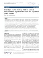
Data encountered in a business environment are more likely to
appear like the data points in this graph, where Y and X
largely obey an approximately linear relationship, but it is not
an exact relationship:

Fig. 1.2
14
12
10

Y

8
6
4
2
0
0

1

2

3

4

5

6

7

X

6 / 42


1. Introduction
2. Approaches to Line Fitting
3. The Least Squares Approach
4. Linear Regression as a Statistical Model
5. Multiple Linear Regression and Matrix Formulation

Introduction

Still, it may be useful to describe the relationship in equation
form, expressing Y as X alone - the equation can be used for
forecasting and policy analysis, allowing for the existence of
errors (since the relationship is not exact).
So how to fit a line to describe the ”broadly linear”
relationship between Y and X when the (x, y ) pairs do not all
lie on a straight line?

7 / 42


1. Introduction
2. Approaches to Line Fitting
3. The Least Squares Approach
4. Linear Regression as a Statistical Model
5. Multiple Linear Regression and Matrix Formulation

Approaches to Line Fitting
Consider the pairs (xi , yi ). Let yˆi be the ”predicted” value of

yi associated with xi if the fitted line is used. Define
ei = yi − yˆi as the residual representing the ”error” involved.

8 / 42


1. Introduction
2. Approaches to Line Fitting
3. The Least Squares Approach
4. Linear Regression as a Statistical Model
5. Multiple Linear Regression and Matrix Formulation

Approaches to Line Fitting
Consider the pairs (xi , yi ). Let yˆi be the ”predicted” value of
yi associated with xi if the fitted line is used. Define
ei = yi − yˆi as the residual representing the ”error” involved.
If over- and under-predictions of the same magnitude are
considered to be equally undesirable, then the object would be
to fit a line to make the absolute error as small as possible,
but noting that the sample contains n observations and given
the relationship is inexact, it would not be possible to
minimise all ei ’s simultaneously.

8 / 42


1. Introduction
2. Approaches to Line Fitting
3. The Least Squares Approach
4. Linear Regression as a Statistical Model

5. Multiple Linear Regression and Matrix Formulation

Approaches to Line Fitting
Consider the pairs (xi , yi ). Let yˆi be the ”predicted” value of
yi associated with xi if the fitted line is used. Define
ei = yi − yˆi as the residual representing the ”error” involved.
If over- and under-predictions of the same magnitude are
considered to be equally undesirable, then the object would be
to fit a line to make the absolute error as small as possible,
but noting that the sample contains n observations and given
the relationship is inexact, it would not be possible to
minimise all ei ’s simultaneously.
Thus, our criterion must be based on some aggregate
measures.
8 / 42


1. Introduction
2. Approaches to Line Fitting
3. The Least Squares Approach
4. Linear Regression as a Statistical Model
5. Multiple Linear Regression and Matrix Formulation

Approaches to Line Fitting
Fig. 1.3
14
12

𝑦𝑦𝑖𝑖

10
8

Y

𝑒𝑒𝑖𝑖

6
4


𝑦𝑦
�𝚤𝚤

2
0
0

1

2

𝑥𝑥𝑖𝑖

3

4

5

6

7

X

9 / 42


1. Introduction
2. Approaches to Line Fitting
3. The Least Squares Approach
4. Linear Regression as a Statistical Model
5. Multiple Linear Regression and Matrix Formulation

Approaches to Line Fitting
Several approaches may be considered:
Eye-balling

10 / 42


1. Introduction
2. Approaches to Line Fitting
3. The Least Squares Approach
4. Linear Regression as a Statistical Model
5. Multiple Linear Regression and Matrix Formulation

Approaches to Line Fitting
Several approaches may be considered:

Eye-balling
Minimise the sum of the errors, i.e.,

n
i=1 ei

=

n
i=1 (yi

− yˆi )

10 / 42


1. Introduction
2. Approaches to Line Fitting
3. The Least Squares Approach
4. Linear Regression as a Statistical Model
5. Multiple Linear Regression and Matrix Formulation

Approaches to Line Fitting
Several approaches may be considered:
Eye-balling
Minimise the sum of the errors, i.e.,

n
i=1 ei

=

n
i=1 (yi

− yˆi )

Minimise the sum of the absolute errors,
n
n
ˆi )|.
i=1 |ei | =
i=1 |(yi − y
Although use of this criterion is gaining popularity, it is not
the one most commonly used because it involves the
application of linear programming. As well, the solution may
not be unique.

10 / 42


1. Introduction
2. Approaches to Line Fitting
3. The Least Squares Approach
4. Linear Regression as a Statistical Model
5. Multiple Linear Regression and Matrix Formulation

The Least Squares Approach
By far, the most common approach to estimating a regression
equation is the least squares approach.

11 / 42


1. Introduction
2. Approaches to Line Fitting
3. The Least Squares Approach
4. Linear Regression as a Statistical Model
5. Multiple Linear Regression and Matrix Formulation

The Least Squares Approach
By far, the most common approach to estimating a regression
equation is the least squares approach.
This approach leads to a fitted line that minimises the sum of
the squared errors, i.e.,
n

n

ei2 =

(yi − yˆi )2
i=1
n

i=1

(yi − b1 − b2 xi )2 .

=

i=1

11 / 42


1. Introduction
2. Approaches to Line Fitting
3. The Least Squares Approach
4. Linear Regression as a Statistical Model
5. Multiple Linear Regression and Matrix Formulation

The Least Squares Approach

To find the values of b1 and b2 that lead to the minimum,
∂

n
2
i=1 ei

∂b1
∂

n
2
i=1 ei

∂b2

n

= −2

(yi − b1 − b2 xi ) = 0

(1)

xi (yi − b1 − b2 xi ) = 0

(2)

i=1
n

= −2
i=1

Equations (1) and (2) are known as normal equations.

12 / 42


1. Introduction
2. Approaches to Line Fitting
3. The Least Squares Approach
4. Linear Regression as a Statistical Model
5. Multiple Linear Regression and Matrix Formulation

The Least Squares Approach
Solving the two normal equations leads to

b2 =

n
¯)(yi −
i=1 (xi − x
n
¯)2
i=1 (xi − x

y¯)

b1 = y¯ − b2 x¯
or
b2 =

n
x y¯
i=1 xi yi − n¯
n
2
x2
i=1 xi − n¯

b1 = y¯ − b2 x¯

13 / 42


1. Introduction
2. Approaches to Line Fitting

3. The Least Squares Approach
4. Linear Regression as a Statistical Model
5. Multiple Linear Regression and Matrix Formulation

The Least Squares Approach

Example 1.1 The cost of adding a new communication node
at a location not currently included in the network is of
concern to a major manufacturing company. To try to predict
the price of new communication nodes, data were observed on
a sample of 14 existing nodes. The installation cost
(Y =COST) and the number of ports available for access
(X =NUMPORTS) in each existing node were available
information.
A scatter plot of the data is shown overleaf.

14 / 42


1. Introduction
2. Approaches to Line Fitting
3. The Least Squares Approach
4. Linear Regression as a Statistical Model
5. Multiple Linear Regression and Matrix Formulation

Approaches to Line Fitting

Fig. 1.4
60000
55000

50000

COST

45000
40000
35000
30000
25000
20000
10

20

30

40

50

60

70

NUMPORTS

15 / 42


1. Introduction

2. Approaches to Line Fitting
3. The Least Squares Approach
4. Linear Regression as a Statistical Model
5. Multiple Linear Regression and Matrix Formulation

The Least Squares Approach
We find
n

xi yi = 23107792,

x¯ = 36.2857,

i=1

y¯ = 40185.5,

n
2
i=1 xi

= 22576

Using our least squares formulae,
23107792 − (14)(36.2857)(40185.5)
22576 − (14)(36.2857)2
= 650.169

b2 =

b1 = 40185.5 − (650.169)36.2857 = 16593.65
The results obtained from EXCEL are shown overleaf.
16 / 42


1. Introduction
2. Approaches to Line Fitting
3. The Least Squares Approach
4. Linear Regression as a Statistical Model
5. Multiple Linear Regression and Matrix Formulation

The Least Squares Approach
Output 1.1: SUMMARY OUTPUT
Regression Statistics
Multiple R
0.941928423
R Square
0.887229154
Adjusted R Square
0.877831584
Standard Error
4306.914458
Observations
14
ANOVA
df
Regression
Residual
Total

Intercept
X Variable 1

1
12
13

SS
1751268376
222594145.8
1973862522

Coefficients
16593.64717
650.1691724

Standard Error
2687.049999
66.91388832

MS
F
1751268376 94.41048161
18549512.15

t Stat
6.17541437
9.716505628

Significance

F
4.88209E-07

P-value
Lower 95%
Upper 95%
4.75984E-05 10739.06816 22448.22618
4.88209E-07 504.3763341 795.9620108

17 / 42