Báo cáo khoa học: Unravelling the functional interaction structure of a cellular network from temporal slope information of experimental data docx
Bạn đang xem bản rút gọn của tài liệu. Xem và tải ngay bản đầy đủ của tài liệu tại đây (412.36 KB, 10 trang )
Unravelling the functional interaction structure of a
cellular network from temporal slope information of
experimental data
Kwang-Hyun Cho
1,2
, Sung-Young Shin
3
and Sang-Mok Choo
3
1 College of Medicine, Seoul National University, Jongno-gu, Seoul, Korea
2 Korea Bio-MAX Institute, Seoul National University, Gwanak-gu, Seoul, Korea
3 School of Electrical Engineering, University of Ulsan, Ulsan, Korea
It is now widely accepted that we need to unravel the
functional interaction structure of the underlying cellu-
lar network (e.g. signalling cascades or gene networks)
in order to get a proper understanding of the biological
function of a living system. Despite the constant
development of new technology, most of the experi-
mental measurements still contain inevitable nonbiolog-
ical variations to some extent [1–4] and it is not always
easy to get enough replicates for statistical preprocess-
ing to eliminate or minimize such nonbiological
Keywords
cellular networks; functional interaction;
structure identification; temporal slope;
time-series data
Correspondence
K H. Cho, Korea Bio-MAX Institute,
3rd Floor, IVI, Seoul National University
Research Park, San 4–8, Bongcheon 7-dong,
Gwanak-gu, Seoul, 151-818, Republic of
Korea
Fax: +82 2 887 2692
Tel: +82 2 887 2650
E-mail:
(Received 16 April 2005, revised 7 June
2005, accepted 13 June 2005)
doi:10.1111/j.1742-4658.2005.04815.x
Due to the unavoidable nonbiological variations accompanying many
experiments, it is imperative to consider a way of unravelling the functional
interaction structure of a cellular network (e.g. signalling cascades or gene
networks) by using the qualitative information of time-series experimental
data instead of computation through the measured absolute values. In this
spirit, we propose a very simple but effective method of identifying the
functional interaction structure of a cellular network based on temporal
ascending or descending slope information from given time-series measure-
ments. From this method, we can gain insight into the acceptable measure-
ment error ranges in order to estimate the correct functional interaction
structure and we can also find guidance for a new experimental design to
complement the insufficient information of a given experimental dataset.
We developed experimental sign equations, making use of the temporal
slope sign information from time-series experimental data, without a speci-
fic assumption on parameter perturbations for each network node. Based
on these equations, we further describe the available specific information
from each part of experimental data in detail and show the functional
interaction structure obtained by integrating such information. In this pro-
cedure, we use only simple algebra on sign changes without complicated
computations on the measured absolute values of the experimental data.
The result is, however, verified through rigorous mathematical definitions
and proofs. The present method provides us with information about the
acceptable measurement error ranges for correct estimation of the func-
tional interaction structure and it further leads to a new experimental
design to complement the given experimental data by informing us about
additional specific sampling points to be chosen for further required infor-
mation.
Abbreviations
HOG, high osmolarity glycerol response; MAP, mitogen-activated protein; MAPK, MAP kinase; MAPKK, MAPK kinase.
3950 FEBS Journal 272 (2005) 3950–3959 ª 2005 FEBS
variations from the experimental data. This makes it
difficult to compute any algorithm or to interpret the
result based on the measured absolute values. Hence,
there is a pressing need to develop a new method
by which we can identify the functional interaction
structure of a cellular network only through the
qualitative information of time-series experimental
data. Motivated by this practical need, we investigate
in this paper a new identification method based on tem-
poral slope changes of the experimental data profiles.
There have been diverse approaches to identify (or
reverse engineer) the functional interaction structure of
a cellular network from given experimental data. These
include using differential equations [5]; linear models
[6]; linear differential equation models [7]; stochastic
models [8]; neural network models [9]; Boolean net-
works [10]; Bayesian networks [11]; dynamic Bayesian
networks [12,13], etc. However, developing a new
method that can unravel the functional interaction
structure based only on the qualitative information of
time-series experimental data remains a challenging
subject.
Other recent important developments include the
identification methods based on parameter perturbation
experiments. In particular, Kholodenko et al. [14] have
proposed a general method for identification of a cellu-
lar network structure based on stationary experimental
data, which is applicable to a network of generalized
modules under the assumption that each module con-
tains at least one intrinsic parameter that can be directly
perturbed without the intervention of other nodes or
parameters. Sontag et al. [15] have proposed another
complementary method based on time-series measure-
ments, which can be useful when stationary data are not
available and the strength of self-regulation at each
node ⁄ module should be estimated as well. It is, however,
only applicable to the case when for each node there are
as many parameters as the number of overall network
nodes and these parameters do not directly affect the
corresponding node. The fundamental concepts of the
methods proposed by Kholodenko et al. [14] and
Sontag et al. [15] have been expounded (K H. Cho,
S M. Choo, P. Wellstead & O. Wolkenhauer, unpub-
lished data) and have presented a comprehensive unified
framework based on the fact that we need n independent
equations to solve n unknowns and these n linearly inde-
pendent equations can be obtained by properly chosen
n parameter perturbations. All these approaches are
based on parameter perturbation experiments which
are, however, not always achievable in many practical
cases.
In this paper, we therefore consider a new identifica-
tion method which does not require parameter pertur-
bation experiments but utilizes only the qualitative
information of time-series experimental data. Specific-
ally, we aim at developing an identification method
based on the temporal slope changes of experimental
data profiles. In other words, we make use of the
information only about temporal ascending or des-
cending slopes from the given time-series experimental
data profiles and do not rely on the measured absolute
values at each sampling time point. This implies that
we require only an experiment that can guarantee such
qualitative information regarding the dynamic pattern
change of time-series profiles and thereby we can also
get insight into the allowable error ranges in the meas-
urements. We can further design a new experiment
through the present approach by gathering informa-
tion about the required sampling time points to ensure
correct dynamic pattern changes. Once we have such
time-series experimental data containing (partially) cor-
rect dynamic pattern changes then we can infer the
(partial) interaction structure of the underlying cellular
network by integrating the analysis results on each
(partial) time interval of measurement. We note here
that only simple algebra on sign changes of the time-
series profiles is used in the present method without
involving any complicated computations on the meas-
ured absolute values of the experimental data. The
result is however, verified through rigorous mathemat-
ical definitions and proofs. The present method is illus-
trated by an artificial example as well as by a simple
real example extracted from the HOG (high osmolarity
glycerol response) pathway for hyperosmolarity adap-
tation in budding yeast (Saccharomyces cerevisiae) and
based on the related mRNA expression time-series
data from Stanford Microarray Databases.
Results
Inferring the functional interaction between
network nodes from dynamic pattern changes
of time-series data
Investigations into the conceptual framework of quan-
tifying molecular interactions in cellular networks
have been getting increasing attention in recent years,
e.g. by Brown et al. [17], Bruggeman et al. [18], and
Kholodenko et al. [19]. Among them, two recent remark-
able developments are that of Kholodenko et al. [14]
based on stationary experimental data, and that of
Sontag et al. [15] based on time-series experimental
data. These two developments have been further
extended and unified (K H. Cho, S M. Choo,
P. Wellstead & O. Wolkenhauer, unpublished data).
All of these methods are however, only applicable to
K H. Cho et al. Identification through temporal slope information
FEBS Journal 272 (2005) 3950–3959 ª 2005 FEBS 3951
the experimental data obtained by parameter perturba-
tions under strict assumptions. As such experiments
are not always achievable due to many practical limita-
tions, we need to consider a new method that can be
applicable to time-series experimental data without
parameter perturbations and that can make use only
of the qualitative information without relying on meas-
ured absolute values. To this end, we first consider the
following dynamic equations for a cellular network:
dx
i
ðtÞ
dt
¼ f
i
x
1
; x
2
; ÁÁÁ; x
n
ðÞ; t 2 0; Tð; i ¼ 1; 2; ÁÁÁ; n ð1Þ
where a variable x
i
is the i
th
network node, denoting the
biochemical quantity of an element, and the corres-
ponding function f
i
describes how the rate of change of
x
i
with respect to (w.r.t.) time depends on all the varia-
bles of the network. From Eqn 1, we can identify the
functional interaction structure of a network if
we reveal the sign of f
ij
xtðÞ½¼
@f
i
xtðÞ½
@x
j
ð1 i; j nÞ at
some time t under the assumption that the sign of
f
ij
[x(t)] is fixed at all time t (i.e. we assume that the func-
tional interaction structure is time-invariant). Specific-
ally, we define that a node j affects a node i if and only
if f
ij
„ 0. In particular, if f
ij
> 0 then we interpret that
the node j activates the node i by increasing the net rate
of x
i
and if f
ij
< 0 then the node j inhibits the node i.
We note that the dynamics of the system in Eqn 1
depend on the initial condition and time lapse, and we
only assume that f
i
(x
1
, x
2
, ÁÁÁ, x
n
)(i ¼ 1, 2, ÁÁÁ,n) is
partially differentiable with respect to all its arguments
x
j
( j ¼ 1, 2, ÁÁÁ, n) (i.e.
@f
i
@x
j
should exist). Hence, we
cannot make use of the information from parameter
perturbations represented by either
dx
i
dp
or
@
2
x
i
@t@p
[14]
and [15], but we can only use the dynamic infor-
mation according to the time lapse, e.g. represented
by
dx
i
dt
, to find the functional interaction structure,
i.e. the sign of f
ij
. As it is difficult to find out the
exact value of
dx
i
dt
from experimental data, we restrict
ourselves to utilizing only the sign of
dx
i
dt
from the
experimental data to identify the sign of f
ij
in the
present method.
For instance, let us consider sample trajectories of
Eqn 1 for n ¼ 2 in Fig. 1A. If we focus only on the
temporal slope changes, there are time points t
a
1
; t
b
1
for which
_
x
1
t
a
1
ÀÁ
> 0 >
_
x
1
t
b
1
ÀÁ
and x
j
t
a
1
ÀÁ
< x
j
t
b
1
ÀÁ
j ¼ 1; 2ðÞ. If we apply the mean value theorem to
_
x
1
¼ f
1
ðx
1
; x
2
Þ w.r.t. t
a
1
and t
b
1
, then we have a theoreti-
cal equation:
D
_
x
i
t
ab
i
ÀÁ
¼
X
n
j¼1
f
ij
ðh
j
ÞÁDx
j
t
ab
i
ÀÁ
ð2Þ
for i ¼ 1 and some h
j
2 R
n
where Dvt
ab
i
ÀÁ
vt
b
i
ÀÁ
À vt
a
i
ÀÁ
6¼ 0. From Eqn 2, we know that
f
11
‡ 0, f
12
‡ 0 are not possible as D
_
x
1
t
ab
1
ÀÁ
< 0;
Dx
j
t
ab
1
ÀÁ
> 0 j ¼ 1; 2ðÞ, and f
11
£ 0, f
12
‡ 0 are also
impossible as D
_
x
1
t
cd
1
ÀÁ
< 0; Dx
1
t
cd
1
ÀÁ
< 0; Dx
2
t
cd
1
ÀÁ
> 0
(Fig. 1). Hence, we can identify the sign of, f
12
, i.e.
f
12
< 0, in this way by excluding such impossible
combinations from all cases. In other words, we first
find the time intervals like Fig. 1A and then identify
the impossible combination of signs in those intervals
as in Fig. 1B by computing the signs of D
_
x
1
t
ab
1
ÀÁ
and
Dx
j
t
ab
1
ÀÁ
j ¼ 1 ; 2ðÞ. Finally, we can identify the sign of
f
12
by integrating all these results. On the other
hand, for identification of the sign of f
11
, we need
to consider another time interval in which we can
identify the remaining impossible sign combinations of
f
11
, f
12
.
Guidance for an experimental design and
allowable measurement error ranges
There have been some fundamental questions regard-
ing an experimental design and measurements to iden-
tify the functional interaction structure of a cellular
network. For instance, how precise the measurement
should be to infer the embedded true interaction lead-
ing to the i
th
node x
i
from the measurement and how
often the measurement should be taken to capture
such a true interaction structure leading to the i
th
node
x
i
from the measured dynamic profiles? Throughout
the investigations into the present method, we can
answer these questions as follows. The experimental
A
B
Fig. 1. Postulated experimental data (A) and an illustration of
impossible cases of the functional interaction structure with regard
to x
1
(B). We can identify the impossible interaction structure by
noting the temporal slope changes at some suitable time sets, e.g.
t
a
1
, t
b
1
ÈÉ
, t
c
1
, t
d
1
ÈÉ
, from the postulated experimental data of the cel-
lular network with two nodes. The arrow indicates an activation
and the line with a bar at its end denotes an inhibition.
Identification through temporal slope information K H. Cho et al.
3952 FEBS Journal 272 (2005) 3950–3959 ª 2005 FEBS
measurement should be taken to provide time-series
data containing some specific time intervals T
i‘
with
t
a
i
; t
b
i
ÂÃ
& T
i‘
where various sign combinations of
D
_
x
j
i
t
ab
i
ÀÁ
and Dx
j
t
ab
i
ÀÁ
are included. Here T
i‘
¼ t
s
i‘
; t
e
i‘
ÂÃ
is called an information interval at x
i
, which contains
three sampling time points t
s
i‘
; t
c
i‘
; t
e
i‘
such that the
temporal profile of x
i
is increasing on t
s
i‘
; t
c
i‘
ÂÃ
and
decreasing on t
c
i‘
; t
e
i‘
ÂÃ
or vice versa, and it is also clear
whether other temporal profiles x
j
(1 £ j £ n, j „ i) are
increasing or decreasing over the same interval T
i‘
.In
the present method, it is assumed that the experimental
measurements are taken only to ensure such informa-
tion intervals for correct estimation of the functional
interaction structure and thereby some measurement
errors are allowed within the ranges accordingly. If a
given experimental data set contains such dynamic
information required to identify the functional inter-
action leading to the i
th
node x
i
, we define the set of
all the information intervals at x
i
as a fully excited
information set at x
i
(Definition 5 in Supplementary
material, Supplementary mathematical descriptions)
and in this case we simply say that the experimental
data set is a fully excited information set at x
i
.
For instance, for the system in Eqns 1 and 2 with
n ¼ 2, if there is an information interval T
11
where the
sign combinations of D
_
x
1
t
ab
1
ÀÁ
; Dx
1
t
ab
1
ÀÁ
; Dx
2
t
ab
1
ÀÁÂÃ
are
(¯,¯,¯), (¯,¯,É), (¯,É,¯) for t
a
1
; t
b
1
ÂÃ
& T
11
, then we
learn that the signs of f
11
, f
12
cannot be any of the
cases among (É,É), ( É,¯), (¯,É), (É,0), (0,É), (¯,0)
and (0,¯). Hence, the signs of f
11
, f
12
turn out to be
(¯,¯). The set {T
11
} is therefore a fully excited infor-
mation set at x
1
in this case.
Given an experimental data set, we can determine
whether it is a fully excited information set at x
i
or not
by applying the present method. If it is not the case
then we can design a new experiment to complement
the given experimental data by finding additional
sampling points to be chosen for the required further
information (Fig. 9). We can, of course, identify a par-
tial interaction structure from the given experimental
data set which is not a fully excited information set at
x
i
without any further experiments (refer to the exam-
ple results in Figs 7 and 8).
Sign equations for identification of the functional
interaction structure
In order to identify the true interaction structure
through the sign of f
ij
based on the information about
temporal slope changes of time-series experimental
data, we first formulate the algebraic Eqn. 2. Given a
fully excited information set at x
i
, we formulate then
the sign equations:
sf
i1
ðÞ6¼
S D
_
x
i
t
ab
i
ÀÁÂÃ
S Dx
1
t
ab
i
ÀÁÂÃ
()
^ÁÁÁ^ sf
in
ðÞ6¼
S D
_
x
i
t
ab
i
ÀÁÂÃ
S Dx
n
t
ab
i
ÀÁÂÃ
()
summarized in Fig. 2 to obtain the impossible network
signs (INS) at x
i
, i.e. the set of all [s( f
i1
) ÁÁÁ,s(f
in
)]
satisfying the sign equations. We note here that s( f
ij
)
(1 £ j £ n) denotes one of the signs among ¯ (‘activa-
tion’), É (‘inhibition’), and 0 (‘no interaction’) for the
unknown sign of f
ij
. We can then obtain the feasible
network signs (FNS) at x
i
by excluding the INS from
the all network signs (ANS) as a complementary set
of the INS in ANS at x
i
(Supplementary material,
Supplementary mathematical descriptions). Note that
S( f
ij
) indicates the sign of f
ij
and [S( f
i1
) ÁÁÁ, S( f
in
)] is
called the true network sign at x
i
, which is included in
the FNS at x
i
.
Based on the information of the FNS at x
i
, we can
find the true network signs. For instance, if the non-
zero s( f
i‘
) in the FNS are all determined as É then
S( f
i‘
) ¼ ¯ (Supplementary material, Supplementary
mathematical descriptions, Theorem 2) while the non-
zero s( f
i‘
) in the FNS are all determined as É then
s( f
i‘
) (Supplementary material, Supplementary mathe-
matical descriptions, Theorem 3). Furthermore, if
there exists both positive and negative signs among
s( f
i‘
) in the FNS at x
i
, then S( f
i‘
) ¼ 0 (Supplementary
material, Supplementary mathematical descriptions,
Theorem 5).
Fig. 2. Determination of the true network
signs through investigation into the INS.
Note the symbol ^ denotes the logical sum,
and the information interval T
i
is a member
of the fully excited information set at x
i
.
K H. Cho et al. Identification through temporal slope information
FEBS Journal 272 (2005) 3950–3959 ª 2005 FEBS 3953
Discussion
Identification of the functional interaction structure
of a cellular network from experimental data has
crucial importance in improving our understanding
on the biological function of a system. In spite of
the recent advancements in this area based on
parameter perturbation experiments such as [14–16],
there has been a practical need to develop a new
identification method without requiring parameter
perturbation experiments but only utilizing the quali-
tative information of time-series experimental data.
In this paper, we have therefore presented a novel
identification method based on temporal slope chan-
ges of the experimental data profiles, which is distin-
guished from any other approaches reported up to
the present. One of the major characteristics of the
presented method is that it can be rather robust to
measurement noise or disturbances since it only
makes use of the qualitative information about tem-
poral ascending or descending slopes from the given
time-series experimental data profiles and does not
rely on the measured absolute value at each samp-
ling time point. This also implies that we can get an
insight into the allowable error ranges in the meas-
urements and can further design a new experiment
such that the required qualitative information regard-
ing the dynamic pattern change of time-series profiles
is guaranteed. The resulting experimental guideline is
quite specific, e.g. by providing us with the informa-
tion about the required sampling time points to cap-
ture correct dynamic pattern changes. We stress here
that only simple algebra on sign changes of the
time-series profiles has been used in the present
method without involving any other complicated
computations on the measured absolute values of the
experimental data. The result has been however, veri-
fied through rigorous mathematical definitions and
proofs.
The proposed method cannot be applied to a case
when the increasing ⁄ decreasing patterns are uncertain
due to noisy variations in experimental data. Hence, in
this case, we need some type of variability information
to set the ‘threshold’ for judging a clear slope change.
One way of dealing with this problem is as follows.
We presume that the experimental data are represented
by some error bars at each sampling time point. If the
error bars of two adjacent sampling time points do not
overlap each other (Fig. 9A) then we define the slope
between these two time points as ‘clear’ since all poss-
ible increasing ⁄ decreasing slope combinations between
the two points should have an identical sign in this
case regardless of the noisy variations. Figure 9A
shows the time-series measurements with error bars
and Fig. 9B illustrates one example profile obtained by
connecting chosen sampled data within the error bars.
We note that the slope information of all possible
dynamic patterns does not change regardless of the
chosen sampled data within the error bars since the
error bars do not overlap in this case.
If some two error bars overlap then the correspond-
ing slope can be uncertain in that there can be a lot of
different increasing ⁄ decreasing slope combinations (i.e.
not all identical signs) between the two points. This
leads then to multiple feasible network signs for each
interaction and we should employ some statistical
measure in this case (e.g. choosing a most frequently
occurring one from the distribution) to decide the most
feasible network sign or some partial interaction struc-
ture, which remains as a further study.
Experimental procedures
Design
The experimental design procedures we propose are as
follows (these are further summarized as a flow diagram
in Fig. 3).
Step 1 – determination of the exact type of temporal
slopes from given time-series experimental data
To determine the correct INS of Fig. 2, the measured time-
series data only need to be precise enough to guarantee the
dynamic patterns, i.e. the temporal ascending or descending
slopes. If the measurements do not satisfy this minimal
requirement, then a new experiment should be designed.
Step 2 – determination of T
i‘
and G
i
First, we find an interval J
i‘
over which the temporal profile
of x
i
increases and then decreases or vice versa. Second, we
choose an interval T
i‘
(‘ ¼ 1 ÁÁÁ, c
i
) among J
i‘
, over which
the signs of Dx
j
t
ab
i
ÀÁ
1 j nðÞis distinct. Then G
i
becomes G
i
¼ {1 ÁÁÁ, c
i
} and {T
i‘
|‘ 2 G
i
} is called an infor-
mation set at x
i
(Supplementary material, Supplementary
mathematical descriptions, Definition 2).
Step 3 – finding the INS at x
i
in Fig. 2
We find [s( f
il
) ÁÁÁ, s( f
in
)] that satisfy the conditions of the
INS at x
i
in Fig. 2 by choosing t
a
i
; t
b
i
over T
i‘
(‘ ¼ 1 ÁÁÁ, c
i
)
such that S
_
x
i
t
a
i
ÀÁÂÃ
Á S
_
x
i
t
b
i
ÀÁÂÃ
< 0 and Dx
j
t
ab
i
ÀÁ
6¼ 0. In this
way, we can exclude the corresponding impossible network
structures.
Identification through temporal slope information K H. Cho et al.
3954 FEBS Journal 272 (2005) 3950–3959 ª 2005 FEBS
Step 4 – finding the true network signs at x
i
in Fig. 2
Provided that the given information set at x
i
is a fully exci-
ted information set at x
i
(Supplementary material, Supple-
mentary mathematical descriptions, Definition 5), we can
find the FNS at x
i
by excluding the INS at x
i
obtained at
Step 3 from the ANS at x
i
and thereby we can identify the
true interaction structure at x
i
(Supplementary material,
Supplementary mathematical descriptions, Theorem 2–5).
In this way, we can still identify a partial interaction struc-
ture even if the given information set at x
i
is not a fully
excited information set at x
i
.
Step 5 – repetition
We can finally identify the overall interaction structure by
repeating the above procedures from Step 2 to Step 4 for
each network node, i(1 £ i £ n).
Illustrative examples
An in-numero example
A network with four nodes
In order to illustrate the present method and to verify its
result, we assume a set of artificial time-series data gen-
erated from a network with a known interaction struc-
ture and known dynamics. For this purpose, we assume
a network composed of four nodes for which
_
m
i
¼
f
i
mðÞi ¼ 1; 2; 3; 4ðÞwhere f
1
(m) ¼ 0.1(m
3
) 1), f
2
(m) ¼
0.1(m
4
) 1), f
3
(m) ¼ –{0.189 + 0.2( m
2
) 1)}(m
1
) 1) and
f
4
(m) ¼ ) 0.1(m
1
) 1)
2
) {0.15–0.1(m
2
) 1)}(m
2
) 1) (Fig. 4A).
To identify the assumed functional interaction structure,
we apply the present method to each time interval of the
generated data profiles where the increasing and the dec-
reasing patterns are distinct. We reorganize the functional
interaction structure by integrating the analysis results and
Fig. 3. Flow diagram of the proposed experi-
mental design procedures (FEIS in Step 2
represents a fully excited information set
and TNS in Step 4 denotes true network
signs).
K H. Cho et al. Identification through temporal slope information
FEBS Journal 272 (2005) 3950–3959 ª 2005 FEBS 3955
then validate the identified structure through comparison
with the assumed original structure. Applying the present
method to this system, we obtain the INS at m
i
in Fig. 5B
from the artificially generated fully excited information set
(Supplementary material, Supplementary impossible network
signs for a detailed example deriving [s( f
i1
) ÁÁÁ, s( f
i4
)]. We
note that the signs of f
1j
, f
2j
(1 £ j £ 4) are fixed in this case.
Hence, we can identify the signs of f
1j
, f
2j
from the FNS sum-
marized in Fig. 5B. That is, S( f
13
) ¼ S( f
24
) ¼ ¯ as s( f
13
)
and s( f
24
) are all fixed with ¯ in the FNS (Supplementary
material, Supplementary mathematical descriptions, Theo-
rem 2), and S( f
1j
) ¼ 0( j ¼ 1, 2, 4) and S( f
2j
) ¼ 0( j ¼ 1, 2, 3)
as the nonzero s( f
1j
)( j ¼ 1, 2, 4) and s( f
2j
)( j ¼ 1, 2, 3) are
variant in the FNS (Supplementary material, Supplementary
mathematical descriptions, Theorem 5).
On the other hand, we note that the signs of f
31
, f
42
are
all É and f
3j
, f
4j
( j ¼ 3, 4) are zero as 0.1 < m
1
< 1.9,
0.1< m
2
< 1.5 in the temporal expression profiles over
(0,300], but the signs of f
32
, f
41
are variant. Thus, we cannot
apply the notion of the fully excited information set to m
3
,
m
4
in this case. Nevertheless we can determine the fixed
signs of f
3j
, f
4j
( j ¼ 3, 4) using the FNS at m
3
, m
4
summar-
ized in Fig. 5B. Applying the present method to the tem-
poral expression profiles in Fig. 5A, we know S( f
3j
) ¼
S( f
4j
) ¼ 0( j ¼ 3, 4) as s( f
3j
), s( f
4j
)( j ¼ 3, 4) vary with ¯
and É in the FNS, and S( f
31
) ¼ S( f
42
) ¼Éas s( f
31
), s( f
42
)
are fixed with É in the FNS (Supplementary material,
Supplementary mathematical descriptions, Theorem 3).
The final, identified interaction structure based on f
ij
from the FNS is depicted in Fig. 6A and the original
postulated interaction structure represented by f
ij
of
_
m
i
¼ f
i
mðÞi ¼ 1; 2; 3; 4ðÞis shown in Fig. 6B. We can
confirm that the identified structure through the present
method is well in accord with the true structure. Although
this simple example illustrates only a four-node case, the
proposed method can be applied to any larger cases in the
AB
Fig. 5. Temporal expression profiles (A) and a summary of the analysis results (B) for the artificial example system. The small circle points
on each temporal profile of m
i
indicate that we can find the corresponding information intervals on the time axis, the number of which is
equal to the number of members in the given fully excited information set at m
i
. The symbol
p
denotes the case that there is (or are)
corresponding one(s) from (f
i1
, f
i2
, f
i3
, f
i4
) (for simplicity, we have omitted the cases that some or all of the f
ij
values are zero in the ANS of
f
ij
at m
i
).
AB
Fig. 4. An artificial model network with four
nodes for the in-numero example (A) and a
simple real example for the partial inter-
action structure of the HOG pathway from
S. cerevisiae (B) for illustration of the
present identification method. The dotted
lines denote the presumed unknown
interaction structure to be identified.
Identification through temporal slope information K H. Cho et al.
3956 FEBS Journal 272 (2005) 3950–3959 ª 2005 FEBS
same manner (Supplementary material, Supplementary feas-
ible network signs: a larger scale artificial example system).
We note however, that the identification of a true inter-
action structure for such larger cases heavily depends
on the available fully excited information set from given
temporal profiles and any a priori biological information on
the functional interactions.
We should consider the dynamic range of the system
when we define an appropriate sampling rate for applica-
tion of the proposed method. The requirement for defining
the sampling rate is to discern the increasing ⁄ decreasing
patterns of the time course profiles. If the given time-series
measurements are uncertain in this respect, another experi-
ment should be designed such that additional sampling time
points are chosen to clarify such uncertain increasing ⁄
decreasing patterns. We note here that the proposed
method is relatively robust with respect to the particular
time points sampled as compared to other methods that
make use of the measured absolute values at each sampling
time point. For instance, the result in Fig. 6 is the same
even if we choose any sampling time points within the time
intervals of (0, 9.6) (46.1, 59.4) (61.4, 75.4) (154.4, 166.1)
(180.8, 193.2) (222.2, 234.1) (270.2, 284.2) rather than the
sampling time points used (i.e. 3.7, 49.2, 69.1, 164.6, 187.2,
232.7, 277.7).
A simple real example
The partial interaction structure of the HOG pathway
in S. cerevisiae
MAP kinase cascades typically composed of three tiers of
protein kinases, a MAP kinase (MAPK), a MAPK kinase
(MAPKK) and a MAPKK kinase (MAPKKK), are
common signalling modules in eukaryotic cells [20,21]. The
budding yeast (S. cerevisiae) has several MAPK cascades
Fig. 6. The identified interaction structure
(A) vs. the original postulated interaction
structure (B) for the artificial example sys-
tem. The dotted lines in A indicate that the
present method is not applicable for identi-
fying these functional interactions. The dual
indications for the signs of f
32
and f
41
in (B)
mean that these functional interactions are
postulated to vary from ¯ into É or vice
versa and thereby S(f
32
) and S(f
41
) are not
identifiable by the present method.
AB
Fig. 7. Temporal expression profiles (A) and a summary of the analysis results (B) for the simple real example system. Note that we cannot
identify the signs of f
1j
(j ¼ 1,2,3) by applying the present method since there is another node (not considered in this model) directly affecting
YPD1 other than YPD1(m
1
), SSK1(m
2
), and SSK2 (m
3
). These are denoted N.A. in (B). Moreover, we learn that additional experiments are
needed to further identify the signs of f
3j
(j ¼ 1,2,3) due to the insufficiently excited information set (IEIS) at m
3
(i.e., the given experimental
data is not a fully excited information set at m
3
in this case).
Fig. 8. The identified partial interaction structure (A) vs. the known
interaction structure from literature (B) for the simple real example
system. The dotted line in A indicates that this functional inter-
action is not identifiable due to the insufficiently excited information
set at m
3
.
K H. Cho et al. Identification through temporal slope information
FEBS Journal 272 (2005) 3950–3959 ª 2005 FEBS 3957
including the HOG response pathway for hyperosmolarity
adaptation [22–26]. Yeast cells respond to increases in extra-
cellular osmolarity by activating the HOG1 MAPK, the
function of which is to elevate the synthesis of glycerol [22].
Extracellular hyperosmolarity in yeast is detected by two
independent transmembrane osmosensors, SHO1 and SLN1.
SHO1 activates the PBS2 (MAPKK) through the STE11
(MAPKKK). Once activated by phosphorylation, PBS2
activates the HOG1 MAPK, which induces glycerol synthe-
sis and other adaptive responses [24,26,27]. SLN1 osmosen-
sor, which is a homologue of prokaryotic two-component
signal transducers, utilizes a multistep phosphorelation
mechanism that involves His and Asp phosphorylation sites
within SLN1, another His phosphorylation site in the inter-
mediary protein YPD1 and an Asp in the receiver domain
protein SSK1 [23,25,26]. SLN1 autophosphorylates under
normal conditions and further phosphorylates YPD1, which
again phosphorylates and de-activates SSK1. Under hyper-
osmotic conditions, SSK1 is not phosphorylated, but acti-
vates the two MAPKKK SSK22 and SSK2, which in turn
activate PBS2 and thereby HOG1 [28]. In this paper, we
consider identification of the two functional interaction
structures between YPD1 and SSK1, and SSK1 and SSK2 ⁄
SSK22 as designated within the box in Fig. 4B (the dotted
lines indicate the presumed unknown interaction structures).
We assume here that the amount of each signalling protein
is proportional to the corresponding mRNA expression
level. Figure 7A shows the temporal gene expression profiles
extracted from the Stanford Microarray Databases (http://
genome-www5.stanford.edu) [29] where m
1
, m
2
, m
3
denote
YPD1, SSK1, SSK2, respectively. Each data point in
Fig. 7A denotes the log
2
-ratio between the measurement
and the reference pool (Experimental data 1) [30] or the
fkh1, 2 asynchronous (Experimental data 2). Note that we
consider only a subset of three molecules from the pathway
for an illustration of applying the proposed method since
the experimental data do not provide the fully excited infor-
mation for the remaining molecules in the pathway.
Note that we cannot identify the functional interactions
leading to m
i
from the given experimental data of m
i
(i ¼
1, 2, 3), as another node (e.g. SLN1 in Fig. 1) other than
m
i
(i ¼ 1, 2, 3) also directly affects m
1
. Regarding the func-
tional interaction leading to m
2
, we can successfully identify
its interaction structure (i.e. the signs of f
2j
( j ¼ 1, 2, 3) from
the given experimental data (Figs 7B and 8A) and can con-
firm that the identified interaction structure is well in accord
with the known result of [26] (Fig. 8 and Supplementary
material, Supplementary impossible network signs for detailed
computation procedures). We note here that the two experi-
ments with different initial conditions contribute to making
the given experimental data into a fully excited information
set with regard to m
2
. We cannot apply the present method
however, to the case of m
3
as there is no T
3‘
that satisfies that
the profile of m
3
is increasing (or decreasing) on the sub-
interval T
1
3‘
of T
3‘
and decreasing (or increasing, respectively)
on the subinterval T
3‘
À T
1
3‘
, and each profile of m
1
and m
2
is also clearly increasing or decreasing on T
3‘
.
Acknowledgements
This work was supported by a grant from the
Korea Ministry of Science and Technology (Korean
Systems Biology Research Grant, M10503010001–
05 N030100111) and by the 21C Frontier Microbial
Genomics and Application Center Program, Ministry
of Science & Technology (Grant MG05-0204-3-0),
Republic of Korea.
References
1 Kerr MK, Martin M & Churchill GA (2000) Analysis
of variance for gene expression microarray data. J Com-
putational Biol 7, 819–837.
2 Vandesompele J, de Preter K, Pattyn F, Poppe B,
van Roy N, de Paepe A & Speleman F (2002) Accurate
normalization of real-time quantitative RT-PCR data
by geometric averaging of multiple internal control
genes. Genome Biol 3, 1–12.
3 Wolkenhauer O, Moller-Levet C & Sanchez-Cabo F
(2002) The curse of normalization. Comparative Func
Genomics 3, 375–379.
Fig. 9. A postulated experimental time-series profile with error bars due to noisy variations (A) vs. one example profile obtained by connect-
ing chosen sampled data within the error bars (B). The slope information of all possible dynamic patterns does not change regardless of the
chosen sampled data within the error bars since the error bars do not overlap in this case. Each interval of (I), (II), and (III) illustrates a con-
ceptual simplification of the temporal slope changes.
Identification through temporal slope information K H. Cho et al.
3958 FEBS Journal 272 (2005) 3950–3959 ª 2005 FEBS
4 Yang YH, Dudoit S, Luu P, Lin DM, Peng V, Ngai J &
Speed TP (2002) Normalization for cDNA microarray
data: A robust composite method addressing single
and multiple slide systematic variation. Nucleic
Acids Res 30, e15.
5 Mestl T, Plahte E & Omholt SW (1995) A mathematical
framework for describing and analysing gene regulatory
networks. J Theor Biol 176, 291–300.
6 D’Haeseleer P, Wen X, Fuhrman S & Somogyi R
(1999) Linear modeling of mRNA expression levels dur-
ing CNS development and injury. Pac Symp Biocomput
4, 41–52.
7 Chen T, He HL & Church GM (1999) Modeling gene
expression with differential equations. Pac Symp Bio-
comput 4, 29–40.
8 Arkin A, Ross J & McAdams HH (1998) Stochastic
kinetic analysis of developmental pathway bifurcation in
phage lambda-infected Escherichia coli cells. Genetics
149, 633–648.
9 Weaver DC, Workman CT & Stormo GD (1999) Mod-
eling regulatory networks with weight matrices. Pac
Symp Biocomput 4 , 112–123.
10 D’Haeseleer P, Liang S & Somogyi R (2000)
Genetic network inference: from co-expression cluster-
ing to reverse engineering. Bioinformatics 16, 707–726.
11 Friedman N, Linial M, Nachman I & Pe’er D (2000)
Using Bayesian networks to analyze expression data.
J Comput Biol 7, 601–620.
12 Ong IM, Glasner JD & Page D (2002) Modelling regu-
latory pathways in E. coli from time series expression
profiles. Bioinformatics 18, S241–S248.
13 Pe’er D, Regev A, Elidan G & Friedman N (2001)
Inferring subnetworks from perturbed expression pro-
files. Bioinformatics 17, S215–S224.
14 Kholodenko BN, Kiyatkin A, Bruggeman FJ, Sontag E,
Westerhoff HV & Hoek JB (2002) Untangling the wires: a
strategy to trace functional interactions in signaling and
gene networks. Proc Natl Acad Sci USA 99, 12841–12846.
15 Sontag E, Kiyatkin A & Kholodenko BN (2004) Infer-
ring dynamic architecture of cellular networks using
time series of gene expression, protein and metabolite
data. Bioinformatics 20, 1877–1886.
16 Reference withdrawn.
17 Brown GC, Hoek JB & Kholodenko BN (1997) Why
do protein kinase cascades have more than one level?
Trends Biochem Sci 22, 288.
18 Bruggeman FJ, Westerhoff HV, Hoek JB &
Kholodenko BN (2002) Modular response analysis of
cellular regulatory networks. J Theor Biol 218, 507–520.
19 Kholodenko BN, Hoek JB, Westerhoff HV & Brown
GC (1997) Quantification of information transfer via
cellular signal transduction pathways. [Erratum (1997)
FEBS Lett. 419, 150] FEBS Lett 414, 430–434.
20 Posas F & Saito H (1998) Activation of the yeast SSK2
MAP kinase kinase kinase by the SSK1 two-component
response regulator. EMBO J 17, 1385–1394.
21 Waskiewicz AJ & Cooper JA (1995) Mitogen and stress
response pathways: MAP kinase cascades and phospha-
tase regulation in mammals and yeast. Curr Opin Cell
Biol 7, 798–805.
22 Brewster JL, de Valoir T, Dwyer ND, Winter E &
Gustin MC (1993) An osmosensing signal transduction
pathway in yeast. Science 259, 1760–1763.
23 Maeda T, Wurgler-Murphy SM & Saito H (1994) A
two-component system that regulates an osmosensing
MAP kinase cascade in yeast. Nature 369, 242–245.
24 Maeda T, Takekawa M & Saito H (1995) Activation
of yeast PBS2 MAPKK by MAPKKKs or by binding
of an SH3-containing osmosensor. Science 269,
554–558.
25 Posas F, Wurgler-Murphy SM, Maeda T, Witten EA,
Thai TC & Saito H (1996) Yeast HOG1 MAP kinase
cascade is regulated by a multistep phosphorelay
mechanism in the SLN1-YPD1-SSK1 ‘two-component’
osmosensor. Cell 86, 865–875.
26 Posas F, Witten EA & Saito H (1998) Requirement of
STE50 for osmostress-induced activation of the STE11
mitogen-activated protein kinase kinase kinase in the
high-osmolarity glycerol response pathway. Mol Cell
Biol 18, 5788–5796.
27 Posas F & Saito H (1997) Osmotic activation of the
HOG MAPK pathway via Ste11p MAPKKK: scaffold
role of Pbs2p MAPKK. Science 276, 1702–1705.
28 Morris PC (2001) MAP kinase signal transduction
pathways in plants. New Phytologist 151, 67–89.
29 Zhu G, Spellman PT, Volpe T, Brown PO, Botstein D,
Davis TN & Futcher B (2000) Two yeast forkhead
genes regulate the cell cycle and pseudohyphal growth.
Nature 406, 90–94.
30 Gasch AP, Spellman PT, Kao CM, Carmel-Harel O,
Eisen MB, Storz G, Botstein D & Brown PO (2000)
Genomic expression programs in the response of yeast
cells to environmental changes. Mol Biol Cell 11, 4241–
4257.
Supplementary material
The following supplementary material is available for
this article online.
Appendix S1 containing the sections: Supplementary
mathematical descriptions; Supplementary impossible
network signs: the artificial example system; Supple-
mentary impossible network signs: the simple real
example system; Supplementary feasible network signs:
a larger scale artificial example system.
K H. Cho et al. Identification through temporal slope information
FEBS Journal 272 (2005) 3950–3959 ª 2005 FEBS 3959