- Trang chủ >>
- Khoa Học Tự Nhiên >>
- Vật lý
Electromagnetism for Electronic Engineers – Examples doc
Bạn đang xem bản rút gọn của tài liệu. Xem và tải ngay bản đầy đủ của tài liệu tại đây (3.15 MB, 156 trang )
Download free ebooks at bookboon.com
2
Richard G. Carter
Electromagnetism for
Electronic Engineers –
Examples
Download free ebooks at bookboon.com
3
Electromagnetism for Electronic Engineers – Examples
© 2010 Richard G. Carter & Ventus Publishing ApS
ISBN 978-87-7681-557-8
Disclaimer: The texts of the advertisements are the sole responsibility of Ventus
Publishing, no endorsement of them by the author is either stated or implied.
Download free ebooks at bookboon.com
Please click the advert
Electromagnetism for Electronic Engineers – Examples
4
Contents
Contents
Preface 6
1 Electrostatics in free space 7
1.1 Introduction 7
1.2 Summary of the methods available 7
2. Dielectric materials and capacitance 35
2.1 Introduction 35
2.2 Summary of the methods available 35
3. Steady electric currents 60
3.1 Introduction 60
3.2 Summary of the methods available 60
4. The magnetic effects of electric currents 76
4.1 Introduction 76
4.2 Summary of the methods available 76
5. The magnetic effects of iron 92
5.1 Introduction 92
5.2 Summary of the methods available 92
6. Electromagnetic induction 115
6.1 Introduction 115
6.2 Summary of the methods available 115
360°
thinking
.
© Deloitte & Touche LLP and affiliated entities.
Discover the truth at www.deloitte.ca/careers
Download free ebooks at bookboon.com
Please click the advert
Electromagnetism for Electronic Engineers – Examples
5
Contents
7. Transmission lines 132
7.1 Introduction 132
7.2 Summary of the methods available 132
8. Maxwell’s equations and electromagnetic waves 150
8.1 Introduction 150
8.2 Summary of the methods available 150
Increase your impact with MSM Executive Education
For more information, visit www.msm.nl or contact us at +31 43 38 70 808
or via
the globally networked management school
For more information, visit www.msm.nl or contact us at +31 43 38 70 808 or via
For almost 60 years Maastricht School of Management has been enhancing the management capacity
of professionals and organizations around the world through state-of-the-art management education.
Our broad range of Open Enrollment Executive Programs offers you a unique interactive, stimulating and
multicultural learning experience.
Be prepared for tomorrow’s management challenges and apply today.
Download free ebooks at bookboon.com
Electromagnetism for Electronic Engineers – Examples
6
Preface
Preface
This is a companion volume to Electromagnetism for Electronic Engineers (3
rd
edn.) (Ventus, 2009).
It contains the worked examples, together with worked solutions to the end of chapter examples,
which featured in the previous edition of the book. I have discovered and corrected a number of
mistakes in the previous edition.
I hope that students will find these 88 worked examples helpful in illustrating how the fundamental
laws of electromagnetism can be applied to a range of problems. I have maintained the emphasis on
examples which may be of practical value and on the assumptions and approximations which are
needed. In many cases the purpose of the calculations is to find the circuit properties of a component
so that the link between the complementary circuit and field descriptions of a problem are illustrated.
Richard Carter
Lancaster 2010
Download free ebooks at bookboon.com
Electromagnetism for Electronic Engineers – Examples
7
1. Electrostatics in free space
1 Electrostatics in free space
1.1 Introduction
Electrostatic problems in free space involve finding the electric fields and the potential distributions
of given arrangements of electrodes. Strictly speaking ‘free space’ means vacuum but the properties
of air and other gases are usually indistinguishable from those of vacuum so it is permissible to
include them in this section. The chief difference is that the breakdown voltage between electrodes
depends upon the gas between them and upon its pressure. The calculation of capacitance between
electrodes in free space is deferred until Chapter 2.
The other problems included in this chapter involve the motion of charged particles (electrons and
ions) in electric fields in vacuum. This topic remains important for certain specialised purposes
including high power radio-frequency and microwave sources, particle accelerators, electron
microscopes, mass spectrometers, ion implantation and electron beam welding and lithography.
1.2 Summary of the methods available
Note: This information is provided here for convenience. The equation numbers in the companion
volume Electromagnetism for Electronic Engineers are indicated by square brackets.
Symbol Signifies Units
i
0
(epsilon) The primary electric constant 8.854 × 10
-12
F.m
-1
Q
Electric charge C
q
Electric line charge C.m
-1
j (sigma) Surface charge density C.m
-2
(rho) Volume charge density C.m
-3
E
Electric field V.m
-1
V
Electric potential V
(del)
The vector differential operator
ˆ
ˆˆˆ
r, x,
y
,z
Unit vectors
Inverse square law of force between charges in free space
12
2
0
ˆ
4
r
Fr [1.1]
Definition of the electric field of a charge in free space
1
2
0
ˆ
4
Q
r
Er [1.2]
Download free ebooks at bookboon.com
Electromagnetism for Electronic Engineers – Examples
8
1. Electrostatics in free space
Force acting on a charge placed in an electric field
2
QFE [1.3]
Gauss’ Theorem
The flux of E out of any closed surface in free space is equal to the charge enclosed by the surface
divided by i
0
.
The integral form of Gauss’ Theorem
0
1
SV
dv
E.dA
[1.5]
The differential form of Gauss’ Theorem
0
.
y
x
z
E
E
E
xyz
E [1.9]
Electrostatic potential difference
B
BA
A
VV
Edl [1.13]
Calculation of electric field from the electrostatic potential
ˆˆˆ
VVV
g
rad V V
xyz
Exyz [1.22]
Poisson’s equation
22 2
2
22 2
0
VVV
V
xyzx
[1.24]
Laplace’s equation
222
2
222
0
VVV
V
xyz
[1.27]
The Principle of Superposition and the method of images
The Principle of conservation of energy
The finite difference method
Download free ebooks at bookboon.com
Electromagnetism for Electronic Engineers – Examples
9
1. Electrostatics in free space
Example 1.1
Find the force on an electron (charge -1.602 × 10
-19
C) which is 1 nm from a perfectly conducting
plane. What is the electric field acting on the electron?
Solution
Using the method of images the conducting plane is replaced by an image charge of +1.602 × 10
-19
C
which is 1 nm behind the position of the conducting plane
The force acting on the electron is found using the inverse square law [1.1] noting that the charges are
2 nm apart.
19 2
(1.602 10 )
12
12
57.7 10 N
22
12 9
4
48.85410 210
0
F
r
(1.1)
Force is a vector quantity so a complete answer must specify its direction. The negative sign indicates
that the electron is attracted to the image charge. The force is therefore acting towards the plane and at
right angles to it.
The electric field acting on the electron is found by substituting its charge and the force acting on it
into [1.3]
12
57.7 10
1
360 MV m
19
1.602 10
F
E
Q
(1.2)
The electric field is a vector quantity and the positive sign indicates that it is acting away from the
plane.
Example 1.2
The surface charge density on a metal electrode is j. Use Gauss’ theorem to show that the electric
field strength close to the surface is
0
E
.
Solution
Consider a small element of area of the surface dA such that the surface around it can be considered to
be a plane. The local charge density can be considered to be constant and, from symmetry
considerations, the electric field must be normal to the conducting surface. Now construct a Gaussian
surface dS, as shown in fig. 1.1, such that it encloses the element dA and has sides which are normal
to the surface and top and bottom faces which are parallel to the surface.
Download free ebooks at bookboon.com
Electromagnetism for Electronic Engineers – Examples
10
1. Electrostatics in free space
dS
dA
E
dh
Fig. 1.1 A Gaussian surface for calculating the electric field of a surface charge.
Since
E is parallel to the sides of dS the flux of E through the sides is zero. Also, because the electric
field within a conducting material is zero when the charges are stationary, the flux of
E through the
bottom of dS is zero. The flux of
E through the top of dS is
dEdA (1.3)
where E is the magnitude of E (since
E is normal to the top of dS). The total charge enclosed by dS is
dQ dA
(1.4)
By Gauss’ theorem
0
dQ
d
(1.5)
Substituting in (1.5) from (1.3) and (1.4) gives
0
E
(1.6)
Note: Because a conducting surface is always an equipotential surface when the charges are stationary
E must always be normal to it. If the surface is curved the electric field varies over it (1.6) shows that,
locally, the charge density is always proportional to the electric field.
Example 1.3
Figure 1.2 right shows a charged wire which is equidistant from a pair of earthed conducting planes
which are at right angles to each other.
a)
Where should image charges be placed in order to solve this problem by the method of images?
b)
What difference would it make if the planes were at 60° to each other?
c)
Could the method be used when the planes were at 50° to each other?
Download free ebooks at bookboon.com
Please click the advert
Electromagnetism for Electronic Engineers – Examples
11
1. Electrostatics in free space
Fig. 1.2 A charged wire close to the intersection of two conducting planes
Solution
a)
If Cartesian co-ordinates are used to describe the positions of the wire and of its images in the
plane then the image line charges are –q at (- d, d) and (d, - d) and +q at (- d, - d) as shown in fig.
1.3.
Get “Bookboon’s Free Media Advice”
See the light!
The sooner you realize we are right,
the sooner your life will get better!
A bit over the top? Yes we know!
We are just that sure that we can make your
media activities more effective.
Download free ebooks at bookboon.com
Electromagnetism for Electronic Engineers – Examples
12
1. Electrostatics in free space
b)
+
+
-
-
Fig. 1.3 Image charges for planes intersecting at 90°
c)
When the planes are at 60° to each other five image charges are equally spaced on a circle as
shown in fig. 1.4.
++
+
-
-
-
Fig. 1.4 Image charges for planes intersecting at 60°
d)
No. The method can only be used when the angle between the planes divides an even number of
times into 360°. Thus it will work for planes at angles of 1/4, 1/6, 1/8, 1/10 of 360° and so on.
Example 1.4
A wire l mm in diameter is placed mid-way between two parallel conducting planes 10 mm apart.
Given that the planes are earthed and the wire is at a potential of 100 V, find a set of image charges
that will enable the electric field pattern to be calculated.
Solution
If we were to put just one image charge on either side of the wire the field pattern could be calculated
by superimposing the fields of the original wire and the image wires. The results would be as shown
in fig.1.5. None of the equipotential surfaces is a plane. The solution is to use an infinite set of equally
spaced wires charged alternately positive and negative, as shown in Fig. 1.6. The symmetry of this set
of wires is such that there must be equipotential planes mid-way between the wires.
Download free ebooks at bookboon.com
Electromagnetism for Electronic Engineers – Examples
13
1. Electrostatics in free space
Fig. 1.5 The field pattern around a positively charged wire flanked by a pair of negatively charged
wires.
Fig. 1.6 The field pattern around a set of equispaced parallel wires charged alternately positive and
negative.
Example 1.5
An air-spaced coaxial line has inner and outer conductors with radii a and b respectively as shown in
fig.1.7. Show that the breakdown voltage of the line is highest when
ln 1ab .
Fig. 1.7: The arrangement of an air-spaced coaxial line
Download free ebooks at bookboon.com
Please click the advert
Electromagnetism for Electronic Engineers – Examples
14
1. Electrostatics in free space
Solution
For most practical purposes the properties of air are indistinguishable from vacuum. From the
symmetry of the problem we note that the electric field must everywhere be radial. The field between
the conducting cylinders is identical to that of a long, uniform, line charge q placed along the axis of
the system.
To find the electric field of a line charge we apply the integral form of Gauss’ equation to a Gaussian
surface consisting of a cylinder of unit length whose radius is r and whose ends are normal to the line
charge as shown in fig.1.8. We note that, from considerations of symmetry, the electric field must be
acting radially outwards and depend only on the radius r.
Fig. 1.8 A Gaussian surface for calculating the electric field strength around a line charge.
S
GOT-THE-ENERGY-TO-LEAD.COM
We believe that energy suppliers should be renewable, too. We are therefore looking for enthusiastic
new colleagues with plenty of ideas who want to join RWE in changing the world. Visit us online to find
out what we are offering and how we are working together to ensure the energy of the future.
Download free ebooks at bookboon.com
Electromagnetism for Electronic Engineers – Examples
15
1. Electrostatics in free space
Let the radial component of the electric field at radius r be E
r
(r). On the curved surface of the cylinder
the radial component of the electric field is constant and the flux is thus the product of the electric
field and the area of the curved surface.
21
r
S
rEr
EdA
(1.7)
The flux of the electric field through the ends of the cylinder is zero because the electric field is
parallel to these surfaces.
We apply Gauss’ theorem [1.5] to find the relationship between the electric field, radius (r) and the
unknown line charge q. Since S has unit length the total charge contained within it, which is denoted
by the right-hand side of [1.5] is just q. Thus
0
2
r
q
rE r
(1.8)
which can be rearranged to give
0
1
2
r
q
Er
r
(1.9)
Since the electric field is inversely proportional to r, it must be greatest when the radius is least, i.e.
when r = a.
max
0
1
2
q
E
a
(1.10)
The potential difference between the cylinders is found from the electric field using [1.13]
00
1
ln
22
b
b
ba r
a
a
qqb
VV Erdr dr
ra
(1.11)
The negative sign tells us that if the charge on the inner cylinder is positive then the electrostatic
potential of the outer cylinder is negative with respect to the inner cylinder.
The unknown charge q can be eliminated between (1.10) and (1.11) to give the potential difference in
terms of the maximum permitted electric field and the dimensions of the line.
max
ln
ba
b
VV Ea
a
(1.12)
Download free ebooks at bookboon.com
Electromagnetism for Electronic Engineers – Examples
16
1. Electrostatics in free space
The condition that the potential difference should be maximum is found by differentiating the
potential difference with respect to the ratio of the dimensions of the conductors and setting the result
to zero. If we set R = b/a the condition can be expressed as
22
ln
11
ln 0
R
d
R
dR R R R
(1.13)
or
ln ln 1Rba (1.14)
Example 1.6
An air-spaced transmission line consists of two parallel cylindrical conductors each 2 mm in diameter
with their centres 10 mm apart as shown in fig. 1.9. Calculate the maximum potential difference
which can be applied to the conductors assuming that the electrical breakdown strength of air
is
1
3MV m
.
Fig. 1.9 A cross-sectional view of a parallel-wire transmission line.
Solution
Since the diameters of the wires are small compared with their separation it is reasonable to assume
that close to the surface of each wire the field pattern is determined almost entirely by that wire. The
equipotential surfaces close to the wires take the form of coaxial cylinders, as may be seen in Fig.
1.10. This is equivalent to assuming that the two wires can be represented by uniform line charges ± q
along their axes. Note that this approximation is only valid if the diameters of the wires are small
compared with the spacing between them.
Download free ebooks at bookboon.com
Please click the advert
Electromagnetism for Electronic Engineers – Examples
17
1. Electrostatics in free space
Fig. 1.10 The field pattern around a parallel-wire transmission line
The electric field of either wire is then given by Equation (1.9) (for r œ1 mm) with the appropriate
sign for q. Since the strength of the electric field of each line charge is inversely proportional to the
distance from the charge, the greatest electric field must occur on the plane passing through the axes
of the two conductors. Using the notation of Fig. 1.9 and Equation (1.9) the electric field on the x axis
between the wires is found by superimposing the fields of the two wires.
11
00
22
22
x
E
dx dx
(1.15)
Contact us to hear more
Who is your target group?
And how can we reach them?
At Bookboon, you can segment the exact right
audience for your advertising campaign.
Our eBooks offer in-book advertising spot to reach
the right candidate.
Download free ebooks at bookboon.com
Electromagnetism for Electronic Engineers – Examples
18
1. Electrostatics in free space
It is easy to show that this expression is a maximum on the inner surfaces of the wires (as might be
expected from Fig. 1.10), that is, when
1
2
x
da . The maximum permissible charge is therefore
given by
max 0 max
2
da
qE
a
d
(1.16)
The potential at points on the x axis between the wires is found from (1.15) using [1.13]
1
2
11 1
00
22 2
ln
22
dx
qqq q
Vx dx C
dx dx dx
(1.17)
where C is a constant of integration. It is convenient to choose C = 0 so that the potential is zero at the
origin.
The maximum permissible potential at A is obtained by substituting the maximum charge from (1.16)
into (1.17) and setting
1
2
x
da to give
max
ln
A
ad a
da
VE
da
(1.18)
The potential at B is -V
A
so the maximum potential difference between the wires is 2V
A
. Substituting
the numbers gives the maximum voltage between the wires as 5.9 kV.
When the wires are not thin compared with their separation the method of solution is similar but, as
can be seen from the equipotentials in Fig. 1.10, the equivalent line charges are no longer located at
the centres of the wires.
Example 1.7
A metal sphere of radius 10 mm is placed with its centre 100 mm from a flat earthed sheet of metal.
Assuming that the breakdown strength of air is 3 MV.m
-1
, calculate the maximum voltage which can
be applied to the electrode without breakdown occurring. What is then the ratio of the maximum to
the mean surface-charge density on the sphere?
Download free ebooks at bookboon.com
Electromagnetism for Electronic Engineers – Examples
19
1. Electrostatics in free space
Solution
This problem is solved using the same procedure as the previous one. It is necessary to assume that
the field is equivalent to that of a pair of point charges placed at the centre of the sphere and of its
image in the plane as shown in fig.1.11. Since the diameter of the sphere is 20% of its distance from
the plane this assumption should not be seriously in error. We note that the attraction between the
surface charges will ensure that the charge density and the electric field are greatest at the point on
each sphere lying closest to the other one.
x
d d
2a
Q -Q
Fig. 1.11 The arrangement of the sphere and its image in the plane.
The first step is to use Gauss’ theorem to find the electric field at a distance r from a point charge Q.
The problem has spherical symmetry and therefore the electric field must be constant on the surface
of a sphere of radius r centred on the charge and directed radially outwards. The surface area of a
sphere of radius r is
2
4 r
so that from [1.5]
2
0
4
r
Q
rE r
(1.19)
so that
2
0
4
r
Q
Er
r
(1.20)
Next we use [1.13] to find the potential at a distance r from the charge.
2
00
44
r
Vr E rdr dr C
rr
(1.21)
where C is a constant of integration. Now
rdx
(1.22)
so that the potential due to the first charge is
Download free ebooks at bookboon.com
Please click the advert
Electromagnetism for Electronic Engineers – Examples
20
1. Electrostatics in free space
0
11
4
Q
Vx C
dx
(1.23)
Similarly the potential due to the other charge is
0
22
4
Q
Vx C
dx
(1.24)
Superimposing the potentials of the two charges gives
00
42
11QQ
x
x
V
dxdx dxdx
(1.25)
At the surface of the first sphere
x
daand
0
22
Qda
Vd a
ada
(1.26) (1.27)
The electric field at the surface of the sphere is found by superimposing the fields of the two charges
using (1.20)
THE BEST MASTER
IN THE NETHERLANDS
Download free ebooks at bookboon.com
Electromagnetism for Electronic Engineers – Examples
21
1. Electrostatics in free space
2
2
0
11
4
2
Q
Ed a
a
da
(1.28)
Eliminating Q between (1.27) and (1.28) gives the relationship between the breakdown field and the
breakdown voltage
1
max max
2
2
11
2
2
2
da
VE
ada a
da
(1.29)
Substituting the numerical values of the quantities we find that the maximum voltage is 28.3 kV
.
From example 1.2 we know that the maximum surface charge density is
12 6 6 2
max 0 max
8.854 10 3 10 26.6 10
E
Cm
(1.30)
The total charge on the sphere can be computed from (1.28)
1
max 0
2
2
11
4
2
QE
a
da
(1.31)
so the average charge density is
11
2
0
max 0 max
22
22
4
11
1
4
22
av
a
EE
aa
da da
(1.32)
and the ratio of peak to average charge density is
2
max
2
1 1.003
2
av
a
da
(1.33)
Example 1.8
An electron starts with zero velocity from a cathode which is at a potential of -10 kV and then moves
into a region of space where the potential is zero. Find its velocity.
Download free ebooks at bookboon.com
Electromagnetism for Electronic Engineers – Examples
22
1. Electrostatics in free space
Solution
The principle of conservation of energy requires that the sum of the kinetic energy and the potential
energy of the electron must be constant. Thus
2
1
0
2
mv qV
(1.34)
where q is the charge on the electron and V is the potential relative to the cathode. The charge to mass
ratio of an electron
11 1
/ 1.759 10 .qm Ckg
and the region of zero potential has a potential relative
to the cathode +10 kV so that, rearranging (1.34) we obtain
11 4 6 -1
2
2 1.759 10 10 59.3 10 m.s
qV
v
m
(1.35)
Note: For accelerating voltages much above 10 kV relativistic effects become important because the
electron velocity is comparable with the velocity of light (0.2998 × 10
9
m s
-1
). It is then necessary to
use the correct relativistic expression for the kinetic energy of the electron, but the principle of the
calculation is unchanged.
Example 1.9
An electron beam originating from a cathode at a potential of -10 kV has a current of 1 A and a radius
of 10 mm. The beam passes along the axis of an earthed conducting cylinder of radius 20 mm as
shown in fig. 1.12. Use Gauss’ theorem to find expressions for the radial electric field within the
cylinder, and calculate the potential on the axis of the system.
r
b
a
x
Electron
beam
Fig. 1.12 The arrangement of an electron beam within a concentric conducting tunnel
Note: Electron beams like this are found in the high power microwave vacuum tubes used in
transmitters for radar, TV broadcasting and satellite communications and for powering particle
accelerators such as the Large Hadron Collider at CERN.
Download free ebooks at bookboon.com
Please click the advert
Electromagnetism for Electronic Engineers – Examples
23
1. Electrostatics in free space
Solution
The velocity of the electrons is given by(1.35). The charge per unit length in an electron beam with
current I and electron velocity v is given by
9-1
16.9 10 C.m
I
q
v
(1.36)
The negative sign arises because the direction of the conventional current is opposite to that of the
electron velocity. If the radius of the beam is b and it is assumed that the current density is uniform
within the beam then
63
2
53.7 10 C.m
q
b
(1.37)
Between the electron beam and the conducting cylinder (region 2) the problem is identical to that in
Example 1.5 and the radial electric field is given by (1.8)
2
0
1
2
q
Er
r
(1.38)
With us you can
shape the future.
Every single day.
For more information go to:
www.eon-career.com
Your energy shapes the future.
Download free ebooks at bookboon.com
Electromagnetism for Electronic Engineers – Examples
24
1. Electrostatics in free space
Within the electron beam (region 1) Gauss’ Theorem can be applied in exactly the same way but the
charge enclosed in unit length of a Gaussian surface of radius r is now
2
qr r
(1.39)
This expression replaces q in (1.38) to give the radial field in region 1
2
0
2
E
rr
(1.40)
The potential in each region is found using [1.13]. In region 1 the result is
11
0
ln
2
q
VrC
(1.41)
The value of C
1
is chosen by requiring V
1
to be zero when r = a so that
1
0
ln
2
qr
V
a
(1.42)
In region 2 we have
2
22
00
24
VrdrrC
(1.43)
The value of C
2
is chosen by setting V
2
= V
1
when r = b.
22
2
00
ln
42
qa
Vbr
b
(1.44)
On the axis r = 0 and
2
2
00
0ln362V
42
qa
Vb
b
(1.45)
Note: This means that the electrons on the axis have a velocity slightly less than that calculated in
(1.35) and electron velocity increases with radius. To obtain an accurate result it would be necessary
to re-compute the electron velocities and the charge density (which now depends on r) to obtain
mutually consistent values.
Download free ebooks at bookboon.com
Electromagnetism for Electronic Engineers – Examples
25
1. Electrostatics in free space
Example 1.10
Figure 1.13 shows a simplified form for the deflection plates for a low current electron beam. Given
that the electron beam is launched from an electrode (the cathode) at a potential of -2000V and passes
between the deflection plates as shown, estimate the angular deflection of the beam when the
potentials of the plates are ±50 V.
Fig. 1.13 The arrangement of a pair of electrostatic deflection plates for an electron beam.
Note: The original use of electrostatic deflection systems in cathode ray tubes for oscilloscopes is now
obsolete but the same system can be used in machines for electron beam lithography, electron beam
welding and scanning electron microscopes.
Solution
To make the problem easier we assume that the electric field is constant everywhere between the
plates and falls abruptly to zero at the ends. Then the field between the plates is found by dividing the
potential difference between the plates by their separation to be E
y
= -5000V m
-1
.
Because there is no x-component of
E, the axial velocity of the electrons is constant and found using
the principle of conservation of energy as in Example 1.8.
6-1
226.510m.s
x
vV
(1.46)
where is the charge to mass ratio of the electron. The time taken for an electron to pass along the
length of the plates (L) is then
1.89 ns
x
L
t
v
(1.47)
The equation of motion in the y direction for an electron is
2
2
y
dy
mqE
dt
(1.48)