Báo cáo khoa học: "Learning to Grade Short Answer Questions using Semantic Similarity Measures and Dependency Graph Alignments" ppt

Proceedings of the 49th Annual Meeting of the Association for Computational Linguistics, pages 752–762,
Portland, Oregon, June 19-24, 2011.
c
2011 Association for Computational Linguistics
Learning to Grade Short Answer Questions using Semantic Similarity
Measures and Dependency Graph Alignments
Michael Mohler
Dept. of Computer Science
University of North Texas
Denton, TX

Razvan Bunescu
School of EECS
Ohio University
Athens, Ohio

Rada Mihalcea
Dept. of Computer Science
University of North Texas
Denton, TX

Abstract
In this work we address the task of computer-
assisted assessment of short student answers.
We combine several graph alignment features
with lexical semantic similarity measures us-
ing machine learning techniques and show
that the student answers can be more accu-
rately graded than if the semantic measures
were used in isolation. We also present a first
attempt to align the dependency graphs of the

student and the instructor answers in order to
make use of a structural component in the au-
tomatic grading of student answers.
1 Introduction
One of the most important aspects of the learning
process is the assessment of the knowledge acquired
by the learner. In a typical classroom assessment
(e.g., an exam, assignment or quiz), an instructor or
a grader provides students with feedback on their
answers to questions related to the subject matter.
However, in certain scenarios, such as a number of
sites worldwide with limited teacher availability, on-
line learning environments, and individual or group
study sessions done outside of class, an instructor
may not be readily available. In these instances, stu-
dents still need some assessment of their knowledge
of the subject, and so, we must turn to computer-
assisted assessment (CAA).
While some forms of CAA do not require sophis-
ticated text understanding (e.g., multiple choice or
true/false questions can be easily graded by a system
if the correct solution is available), there are also stu-
dent answers made up of free text that may require
textual analysis. Research to date has concentrated
on two subtasks of CAA: grading essay responses,
which includes checking the style, grammaticality,
and coherence of the essay (Higgins et al., 2004),
and the assessment of short student answers (Lea-
cock and Chodorow, 2003; Pulman and Sukkarieh,
2005; Mohler and Mihalcea, 2009), which is the fo-

cus of this work.
An automatic short answer grading system is one
that automatically assigns a grade to an answer pro-
vided by a student, usually by comparing it to one
or more correct answers. Note that this is different
from the related tasks of paraphrase detection and
textual entailment, since a common requirement in
student answer grading is to provide a grade on a
certain scale rather than make a simple yes/no deci-
sion.
In this paper, we explore the possibility of im-
proving upon existing bag-of-words (BOW) ap-
proaches to short answer grading by utilizing ma-
chine learning techniques. Furthermore, in an at-
tempt to mirror the ability of humans to understand
structural (e.g. syntactic) differences between sen-
tences, we employ a rudimentary dependency-graph
alignment module, similar to those more commonly
used in the textual entailment community.
Specifically, we seek answers to the following
questions. First, to what extent can machine learn-
ing be leveraged to improve upon existing ap-
proaches to short answer grading. Second, does the
dependency parse structure of a text provide clues
that can be exploited to improve upon existing BOW
methodologies?
752
2 Related Work
Several state-of-the-art short answer grading sys-
tems (Sukkarieh et al., 2004; Mitchell et al., 2002)

require manually crafted patterns which, if matched,
indicate that a question has been answered correctly.
If an annotated corpus is available, these patterns
can be supplemented by learning additional pat-
terns semi-automatically. The Oxford-UCLES sys-
tem (Sukkarieh et al., 2004) bootstraps patterns by
starting with a set of keywords and synonyms and
searching through windows of a text for new pat-
terns. A later implementation of the Oxford-UCLES
system (Pulman and Sukkarieh, 2005) compares
several machine learning techniques, including in-
ductive logic programming, decision tree learning,
and Bayesian learning, to the earlier pattern match-
ing approach, with encouraging results.
C-Rater (Leacock and Chodorow, 2003) matches
the syntactical features of a student response (i.e.,
subject, object, and verb) to that of a set of correct
responses. This method specifically disregards the
BOW approach to take into account the difference
between “dog bites man” and “man bites dog” while
still trying to detect changes in voice (i.e., “the man
was bitten by the dog”).
Another short answer grading system, AutoTutor
(Wiemer-Hastings et al., 1999), has been designed
as an immersive tutoring environment with a graph-
ical “talking head” and speech recognition to im-
prove the overall experience for students. AutoTutor
eschews the pattern-based approach entirely in favor
of a BOW LSA approach (Landauer and Dumais,
1997). Later work on AutoTutor(Wiemer-Hastings

et al., 2005; Malatesta et al., 2002) seeks to expand
upon their BOW approach which becomes less use-
ful as causality (and thus word order) becomes more
important.
A text similarity approach was taken in (Mohler
and Mihalcea, 2009), where a grade is assigned
based on a measure of relatedness between the stu-
dent and the instructor answer. Several measures are
compared, including knowledge-based and corpus-
based measures, with the best results being obtained
with a corpus-based measure using Wikipedia com-
bined with a “relevance feedback” approach that it-
eratively augments the instructor answer by inte-
grating the student answers that receive the highest
grades.
In the dependency-based classification compo-
nent of the Intelligent Tutoring System (Nielsen et
al., 2009), instructor answers are parsed, enhanced,
and manually converted into a set of content-bearing
dependency triples or facets. For each facet of the
instructor answer each student’s answer is labelled
to indicate whether it has addressed that facet and
whether or not the answer was contradictory. The
system uses a decision tree trained on part-of-speech
tags, dependency types, word count, and other fea-
tures to attempt to learn how best to classify an an-
swer/facet pair.
Closely related to the task of short answer grading
is the task of textual entailment (Dagan et al., 2005),
which targets the identification of a directional in-

ferential relation between texts. Given a pair of two
texts as input, typically referred to as text and hy-
pothesis, a textual entailment system automatically
finds if the hypothesis is entailed by the text.
In particular, the entailment-related works that are
most similar to our own are the graph matching tech-
niques proposed by Haghighi et al. (2005) and Rus
et al. (2007). Both input texts are converted into a
graph by using the dependency relations obtained
from a parser. Next, a matching score is calculated,
by combining separate vertex- and edge-matching
scores. The vertex matching functions use word-
level lexical and semantic features to determine the
quality of the match while the the edge matching
functions take into account the types of relations and
the difference in lengths between the aligned paths.
Following the same line of work in the textual en-
tailment world are (Raina et al., 2005), (MacCartney
et al., 2006), (de Marneffe et al., 2007), and (Cham-
bers et al., 2007), which experiment variously with
using diverse knowledge sources, using a perceptron
to learn alignment decisions, and exploiting natural
logic.
3 Answer Grading System
We use a set of syntax-aware graph alignment fea-
tures in a three-stage pipelined approach to short an-
swer grading, as outlined in Figure 1.
In the first stage (Section 3.1), the system is pro-
vided with the dependency graphs for each pair of
instructor (A

i
) and student (A
s
) answers. For each
753
Figure 1: Pipeline model for scoring short-answer pairs.
node in the instructor’s dependency graph, we com-
pute a similarity score for each node in the student’s
dependency graph based upon a set of lexical, se-
mantic, and syntactic features applied to both the
pair of nodes and their corresponding subgraphs.
The scoring function is trained on a small set of man-
ually aligned graphs using the averaged perceptron
algorithm.
In the second stage (Section 3.2), the node simi-
larity scores calculated in the previous stage are used
to weight the edges in a bipartite graph representing
the nodes in A
i
on one side and the nodes in A
s
on
the other. We then apply the Hungarian algorithm
to find both an optimal matching and the score asso-
ciated with such a matching. In this stage, we also
introduce question demoting in an attempt to reduce
the advantage of parroting back words provided in
the question.
In the final stage (Section 3.4), we produce an
overall grade based upon the alignment scores found

in the previous stage as well as the results of several
semantic BOW similarity measures (Section 3.3).
Using each of these as features, we use Support Vec-
tor Machines (SVM) to produce a combined real-
number grade. Finally, we build an Isotonic Regres-
sion (IR) model to transform our output scores onto
the original [0,5] scale for ease of comparison.
3.1 Node to Node Matching
Dependency graphs for both the student and in-
structor answers are generated using the Stanford
Dependency Parser (de Marneffe et al., 2006) in
collapse/propagate mode. The graphs are further
post-processed to propagate dependencies across the
“APPOS” (apposition) relation, to explicitly encode
negation, part-of-speech, and sentence ID within
each node, and to add an overarching ROOT node
governing the main verb or predicate of each sen-
tence of an answer. The final representation is a
list of (relation,governor,dependent) triples, where
governor and dependent are both tokens described
by the tuple (sentenceID:token:POS:wordPosition).
For example: (nsubj, 1:provide:VBZ:4, 1:pro-
gram:NN:3) indicates that the noun “program” is a
subject in sentence 1 whose associated verb is “pro-
vide.”
If we consider the dependency graphs output by
the Stanford parser as directed (minimally cyclic)
graphs,
1
we can define for each node x a set of nodes

N
x
that are reachable from x using a subset of the
relations (i.e., edge types)
2
. We variously define
“reachable” in four ways to create four subgraphs
defined for each node. These are as follows:
• N
0
x
: All edge types may be followed
• N
1
x
: All edge types except for subject types,
ADVCL, PURPCL, APPOS, PARATAXIS,
ABBREV, TMOD, and CONJ
• N
2
x
: All edge types except for those in N
1
x
plus
object/complement types, PREP, and RCMOD
• N
3
x
: No edge types may be followed (This set

is the single starting node x)
Subgraph similarity (as opposed to simple node
similarity) is a means to escape the rigidity involved
in aligning parse trees while making use of as much
of the sentence structure as possible. Humans intu-
itively make use of modifiers, predicates, and subor-
dinate clauses in determining that two sentence en-
tities are similar. For instance, the entity-describing
phrase “men who put out fires” matches well with
“firemen,” but the words “men” and “firemen” have
1
The standard output of the Stanford Parser produces rooted
trees. However, the process of collapsing and propagating de-
pendences violates the tree structure which results in a tree
with a few cross-links between distinct branches.
2
For more information on the relations used in this experi-
ment, consult the Stanford Typed Dependencies Manual at
/>manual.pdf
754
less inherent similarity. It remains to be determined
how much of a node’s subgraph will positively en-
rich its semantics. In addition to the complete N
0
x
subgraph, we chose to include N
1
x
and N
2

x
as tight-
ening the scope of the subtree by first removing
more abstract relations, then sightly more concrete
relations.
We define a total of 68 features to be used to train
our machine learning system to compute node-node
(more specifically, subgraph-subgraph) matches. Of
these, 36 are based upon the semantic similarity
of four subgraphs defined by N
[0 3]
x
. All eight
WordNet-based similarity measures listed in Sec-
tion 3.3 plus the LSA model are used to produce
these features. The remaining 32 features are lexico-
syntactic features
3
defined only for N
3
x
and are de-
scribed in more detail in Table 2.
We use φ(x
i
, x
s
) to denote the feature vector as-
sociated with a pair of nodes x
i

, x
s
, where x
i
is
a node from the instructor answer A
i
and x
s
is a
node from the student answer A
s
. A matching score
can then be computed for any pair x
i
, x
s
 ∈ A
i
×
A
s
through a linear scoring function f(x
i
, x
s
) =
w
T
φ(x

i
, x
s
). In order to learn the parameter vec-
tor w, we use the averaged version of the percep-
tron algorithm (Freund and Schapire, 1999; Collins,
2002).
As training data, we randomly select a subset of
the student answers in such a way that our set was
roughly balanced between good scores, mediocre
scores, and poor scores. We then manually annotate
each node pair x
i
, x
s
 as matching, i.e. A(x
i
, x
s
) =
+1, or not matching, i.e. A(x
i
, x
s
) = −1. Overall,
32 student answers in response to 21 questions with
a total of 7303 node pairs (656 matches, 6647 non-
matches) are manually annotated. The pseudocode
for the learning algorithm is shown in Table 1. Af-
ter training the perceptron, these 32 student answers

are removed from the dataset, not used as training
further along in the pipeline, and are not included in
the final results. After training for 50 epochs,
4
the
matching score f(x
i
, x
s
) is calculated (and cached)
for each node-node pair across all student answers
for all assignments.
3
Note that synonyms include negated antonyms (and vice
versa). Hypernymy and hyponymy are restricted to at most
two steps).
4
This value was chosen arbitrarily and was not tuned in anyway
0. set w ← 0, w ← 0, n ← 0
1. repeat for T epochs:
2. foreach A
i
; A
s
:
3. foreach x
i
, x
s
 ∈ A

i
× A
s
:
4. if sgn(w
T
φ(x
i
, x
s
)) = sgn(A(x
i
, x
s
)):
5. set w ← w + A(x
i
, x
s
)φ(x
i
, x
s
)
6. set w ← w + w, n ← n + 1
7. return w/n.
Table 1: Perceptron Training for Node Matching.
3.2 Graph to Graph Alignment
Once a score has been computed for each node-node
pair across all student/instructor answer pairs, we at-

tempt to find an optimal alignment for the answer
pair. We begin with a bipartite graph where each
node in the student answer is represented by a node
on the left side of the bipartite graph and each node
in the instructor answer is represented by a node
on the right side. The score associated with each
edge is the score computed for each node-node pair
in the previous stage. The bipartite graph is then
augmented by adding dummy nodes to both sides
which are allowed to match any node with a score of
zero. An optimal alignment between the two graphs
is then computed efficiently using the Hungarian al-
gorithm. Note that this results in an optimal match-
ing, not a mapping, so that an individual node is as-
sociated with at most one node in the other answer.
At this stage we also compute several alignment-
based scores by applying various transformations to
the input graphs, the node matching function, and
the alignment score itself.
The first and simplest transformation involves the
normalization of the alignment score. While there
are several possible ways to normalize a matching
such that longer answers do not unjustly receive
higher scores, we opted to simply divide the total
alignment score by the number of nodes in the in-
structor answer.
The second transformation scales the node match-
ing score by multiplying it with the idf
5
of the in-

structor answer node, i.e., replace f(x
i
, x
s
) with
idf(x
i
) ∗ f(x
i
, x
s
).
The third transformation relies upon a certain
real-world intuition associated with grading student
5
Inverse document frequency, as computed from the British Na-
tional Corpus (BNC)
755
Name Type # features Description
RootMatch binary 5 Is a ROOT node matched to: ROOT, N, V, JJ, or Other
Lexical binary 3 Exact match, Stemmed match, close Levenshtein match
POSMatch
binary 2 Exact POS match, Coarse POS match
POSPairs binary 8 Specific X-Y POS matches found
Ontological
binary 4 WordNet relationships: synonymy, antonymy, hypernymy, hyponymy
RoleBased binary 3 Has as a child - subject, object, verb
VerbsSubject binary 3 Both are verbs and neither, one, or both have a subject child
VerbsObject
binary 3 Both are verbs and neither, one, or both have an object child

Semantic real 36 Nine semantic measures across four subgraphs each
Bias constant 1 A value of 1 for all vectors
Total 68
Table 2: Subtree matching features used to train the perceptron
answers – repeating words in the question is easy
and is not necessarily an indication of student under-
standing. With this in mind, we remove any words
in the question from both the instructor answer and
the student answer.
In all, the application of the three transforma-
tions leads to eight different transform combina-
tions, and therefore eight different alignment scores.
For a given answer pair (A
i
, A
s
), we assemble the
eight graph alignment scores into a feature vector
ψ
G
(A
i
, A
s
).
3.3 Lexical Semantic Similarity
Haghighi et al. (2005), working on the entailment
detection problem, point out that finding a good
alignment is not sufficient to determine that the
aligned texts are in fact entailing. For instance, two

identical sentences in which an adjective from one is
replaced by its antonym will have very similar struc-
tures (which indicates a good alignment). However,
the sentences will have opposite meanings. Further
information is necessary to arrive at an appropriate
score.
In order to address this, we combine the graph
alignment scores, which encode syntactic knowl-
edge, with the scores obtained from semantic sim-
ilarity measures.
Following Mihalcea et al. (2006) and Mohler
and Mihalcea (2009), we use eight knowledge-
based measures of semantic similarity: shortest path
[PATH], Leacock & Chodorow (1998) [LCH], Lesk
(1986), Wu & Palmer(1994) [WUP], Resnik (1995)
[RES], Lin (1998), Jiang & Conrath (1997) [JCN],
Hirst & St. Onge (1998) [HSO], and two corpus-
based measures: Latent Semantic Analysis [LSA]
(Landauer and Dumais, 1997) and Explicit Seman-
tic Analysis [ESA] (Gabrilovich and Markovitch,
2007).
Briefly, for the knowledge-based measures, we
use the maximum semantic similarity – for each
open-class word – that can be obtained by pairing
it up with individual open-class words in the sec-
ond input text. We base our implementation on
the WordNet::Similarity package provided by Ped-
ersen et al. (2004). For the corpus-based measures,
we create a vector for each answer by summing
the vectors associated with each word in the an-

swer – ignoring stopwords. We produce a score in
the range [0 1] based upon the cosine similarity be-
tween the student and instructor answer vectors. The
LSA model used in these experiments was built by
training Infomap
6
on a subset of Wikipedia articles
that contain one or more common computer science
terms. Since ESA uses Wikipedia article associa-
tions as vector features, it was trained using a full
Wikipedia dump.
3.4 Answer Ranking and Grading
We combine the alignment scores ψ
G
(A
i
, A
s
) with
the scores ψ
B
(A
i
, A
s
) from the lexical seman-
tic similarity measures into a single feature vector
ψ(A
i
, A

s
) = [ψ
G
(A
i
, A
s
)|ψ
B
(A
i
, A
s
)]. The fea-
ture vector ψ
G
(A
i
, A
s
) contains the eight alignment
scores found by applying the three transformations
in the graph alignment stage. The feature vector
ψ
B
(A
i
, A
s
) consists of eleven semantic features –

the eight knowledge-based features plus LSA, ESA
and a vector consisting only of tf*idf weights – both
with and without question demoting. Thus, the en-
tire feature vector ψ(A
i
, A
s
) contains a total of 30
features.
6
/>756
An input pair (A
i
, A
s
) is then associated with a
grade g(A
i
, A
s
) = u
T
ψ(A
i
, A
s
) computed as a lin-
ear combination of features. The weight vector u is
trained to optimize performance in two scenarios:
Regression: An SVM model for regression (SVR)

is trained using as target function the grades as-
signed by the instructors. We use the libSVM
7
im-
plementation of SVR, with tuned parameters.
Ranking: An SVM model for ranking (SVMRank)
is trained using as ranking pairs all pairs of stu-
dent answers (A
s
, A
t
) such that grade(A
i
, A
s
) >
grade(A
i
, A
t
), where A
i
is the corresponding in-
structor answer. We use the SVMLight
8
implemen-
tation of SVMRank with tuned parameters.
In both cases, the parameters are tuned using a
grid-search. At each grid point, the training data is
partitioned into 5 folds which are used to train a tem-

porary SVM model with the given parameters. The
regression passage selects the grid point with the
minimal mean square error (MSE), and the SVM-
Rank package tries to minimize the number of dis-
cordant pairs. The parameters found are then used to
score the test set – a set not used in the grid training.
3.5 Isotonic Regression
Since the end result of any grading system is to give
a student feedback on their answers, we need to en-
sure that the system’s final score has some mean-
ing. With this in mind, we use isotonic regression
(Zadrozny and Elkan, 2002) to convert the system
scores onto the same [0 5] scale used by the an-
notators. This has the added benefit of making the
system output more directly related to the annotated
grade, which makes it possible to report root mean
square error in addition to correlation. We train the
isotonic regression model on each type of system
output (i.e., alignment scores, SVM output, BOW
scores).
4 Data Set
To evaluate our method for short answer grading,
we created a data set of questions from introductory
computer science assignments with answers pro-
vided by a class of undergraduate students. The as-
signments were administered as part of a Data Struc-
7
/>8
/>tures course at the University of North Texas. For
each assignment, the student answers were collected

via an online learning environment.
The students submitted answers to 80 questions
spread across ten assignments and two examina-
tions.
9
Table 3 shows two question-answer pairs
with three sample student answers each. Thirty-one
students were enrolled in the class and submitted an-
swers to these assignments. The data set we work
with consists of a total of 2273 student answers. This
is less than the expected 31 × 80 = 2480 as some
students did not submit answers for a few assign-
ments. In addition, the student answers used to train
the perceptron are removed from the pipeline after
the perceptron training stage.
The answers were independently graded by two
human judges, using an integer scale from 0 (com-
pletely incorrect) to 5 (perfect answer). Both human
judges were graduate students in the computer sci-
ence department; one (grader1) was the teaching as-
sistant assigned to the Data Structures class, while
the other (grader2) is one of the authors of this pa-
per. We treat the average grade of the two annotators
as the gold standard against which we compare our
system output.
Difference Examples % of examples
0 1294 57.7%
1 514 22.9%
2 231 10.3%
3 123 5.5%

4 70 3.1%
5 9 0.4%
Table 4: Annotator Analysis
The annotators were given no explicit instructions
on how to assign grades other than the [0 5] scale.
Both annotators gave the same grade 57.7% of the
time and gave a grade only 1 point apart 22.9% of
the time. The full breakdown can be seen in Table
4. In addition, an analysis of the grading patterns
indicate that the two graders operated off of differ-
ent grading policies where one grader (grader1) was
more generous than the other. In fact, when the two
differed, grader1 gave the higher grade 76.6% of the
time. The average grade given by grader1 is 4.43,
9
Note that this is an expanded version of the dataset used by
Mohler and Mihalcea (2009)
757
Sample questions, correct answers, and student answers Grades
Question: What is the role of a prototype program in problem solving?
Correct answer: To simulate the behavior of portions of the desired software product.
Student answer 1: A prototype program is used in problem solving to collect data for the problem. 1, 2
Student answer 2:
It simulates the behavior of portions of the desired software product. 5, 5
Student answer 3:
To find problem and errors in a program before it is finalized. 2, 2
Question: What are the main advantages associated with object-oriented programming?
Correct answer: Abstraction and reusability.
Student answer 1: They make it easier to reuse and adapt previously written code and they separate complex
programs into smaller, easier to understand classes. 5, 4

Student answer 2:
Object oriented programming allows programmers to use an object with classes that can be
changed and manipulated while not affecting the entire object at once. 1, 1
Student answer 3:
Reusable components, Extensibility, Maintainability, it reduces large problems into smaller
more manageable problems. 4, 4
Table 3: A sample question with short answers provided by students and the grades assigned by the two human judges
while the average grade given by grader2 is 3.94.
The dataset is biased towards correct answers. We
believe all of these issues correctly mirror real-world
issues associated with the task of grading.
5 Results
We independently test two components of our over-
all grading system: the node alignment detection
scores found by training the perceptron, and the
overall grades produced in the final stage. For the
alignment detection, we report the precision, recall,
and F-measure associated with correctly detecting
matches. For the grading stage, we report a single
Pearson’s correlation coefficient tracking the anno-
tator grades (average of the two annotators) and the
output score of each system. In addition, we re-
port the Root Mean Square Error (RMSE) for the
full dataset as well as the median RMSE across each
individual question. This is to give an indication of
the performance of the system for grading a single
question in isolation.
10
5.1 Perceptron Alignment
For the purpose of this experiment, the scores as-

sociated with a given node-node matching are con-
verted into a simple yes/no matching decision where
positive scores are considered a match and negative
10
We initially intended to report an aggregate of question-level
Pearson correlation results, but discovered that the dataset
contained one question for which each student received full
points – leaving the correlation undefined. We believe that
this casts some doubt on the applicability of Pearson’s (or
Spearman’s) correlation coefficient for the short answer grad-
ing task. We have retained its use here alongside RMSE for
ease of comparison.
scores a non-match. The threshold weight learned
from the bias feature strongly influences the point
at which real scores change from non-matches to
matches, and given the threshold weight learned by
the algorithm, we find an F-measure of 0.72, with
precision(P) = 0.85 and recall(R) = 0.62. However,
as the perceptron is designed to minimize error rate,
this may not reflect an optimal objective when seek-
ing to detect matches. By manually varying the
threshold, we find a maximum F-measure of 0.76,
with P=0.79 and R=0.74. Figure 2 shows the full
precision-recall curve with the F-measure overlaid.
0
0.2
0.4
0.6
0.8
1

0 0.2 0.4 0.6 0.8 1
Score
Recall
Precision
F-Measure
Threshold
Figure 2: Precision, recall, and F-measure on node-level
match detection
5.2 Question Demoting
One surprise while building this system was the con-
sistency with which the novel technique of question
demoting improved scores for the BOW similarity
measures. With this relatively minor change the av-
erage correlation between the BOW methods’ sim-
758
ilarity scores and the student grades improved by
up to 0.046 with an average improvement of 0.019
across all eleven semantic features. Table 5 shows
the results of applying question demoting to our
semantic features. When comparing scores using
RMSE, the difference is less consistent, yielding an
average improvement of 0.002. However, for one
measure (tf*idf), the improvement is 0.063 which
brings its RMSE score close to the lowest of all
BOW metrics. The reasons for this are not entirely
clear. As a baseline, we include here the results of
assigning the average grade (as determined on the
training data) for each question. The average grade
was chosen as it minimizes the RMSE on the train-
ing data.

ρ w/ QD RMSE w/ QD Med. RMSE w/ QD
Lesk 0.450 0.462 1.034 1.050 0.930 0.919
JCN 0.443 0.461 1.022 1.026 0.954 0.923
HSO 0.441 0.456 1.036 1.034 0.966 0.935
PATH 0.436 0.457 1.029 1.030 0.940 0.918
RES 0.409 0.431 1.045 1.035 0.996 0.941
Lin 0.382 0.407 1.069 1.056 0.981 0.949
LCH 0.367 0.387 1.068 1.069 0.986 0.958
WUP 0.325 0.343 1.090 1.086 1.027 0.977
ESA 0.395 0.401 1.031 1.086 0.990 0.955
LSA 0.328 0.335 1.065 1.061 0.951 1.000
tf*idf 0.281 0.327 1.085 1.022 0.991 0.918
Avg.grade 1.097 1.097 0.973 0.973
Table 5: BOW Features with Question Demoting (QD).
Pearson’s correlation, root mean square error (RMSE),
and median RMSE for all individual questions.
5.3 Alignment Score Grading
Before applying any machine learning techniques,
we first test the quality of the eight graph alignment
features ψ
G
(A
i
, A
s
) independently. Results indicate
that the basic alignment score performs comparably
to most BOW approaches. The introduction of idf
weighting seems to degrade performance somewhat,
while introducing question demoting causes the cor-

relation with the grader to increase while increasing
RMSE somewhat. The four normalized components
of ψ
G
(A
i
, A
s
) are reported in Table 6.
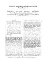
5.4 SVM Score Grading
The SVM components of the system are run on the
full dataset using a 12-fold cross validation. Each of
the 10 assignments and 2 examinations (for a total
of 12 folds) is scored independently with ten of the
remaining eleven used to train the machine learn-
Standard w/ IDF w/ QD w/ QD+IDF
Pearson’s ρ 0.411 0.277 0.428 0.291
RMSE 1.018 1.078 1.046 1.076
Median RMSE 0.910 0.970 0.919 0.992
Table 6: Alignment Feature/Grade Correlations using
Pearson’s ρ. Results are also reported when inverse doc-
ument frequency weighting (IDF) and question demoting
(QD) are used.
ing system. For each fold, one additional fold is
held out for later use in the development of an iso-
tonic regression model (see Figure 3). The param-
eters (for cost C and tube width ǫ) were found us-
ing a grid search. At each point on the grid, the data
from the ten training folds was partitioned into 5 sets
which were scored according to the current param-

eters. SVMRank and SVR sought to minimize the
number of discordant pairs and the mean absolute
error, respectively.
Both SVM models are trained using a linear ker-
nel.
11
Results from both the SVR and the SVMRank
implementations are reported in Table 7 along with
a selection of other measures. Note that the RMSE
score is computed after performing isotonic regres-
sion on the SVMRank results, but that it was unnec-
essary to perform an isotonic regression on the SVR
results as the system was trained to produce a score
on the correct scale.
We report the results of running the systems on
three subsets of features ψ(A
i
, A
s
): BOW features
ψ
B
(A
i
, A
s
) only, alignment features ψ
G
(A
i

, A
s
)
only, or the full feature vector (labeled “Hybrid”).
Finally, three subsets of the alignment features are
used: only unnormalized features, only normalized
features, or the full alignment feature set.
B CA − Ten Folds
B CA − Ten Folds
B CA − Ten FoldsIR Model
SVM Model
Features
Figure 3: Dependencies of the SVM/IR training stages.
11
We also ran the SVR system using quadratic and radial-basis
function (RBF) kernels, but the results did not show signifi-
cant improvement over the simpler linear kernel.
759
Unnormalized Normalized Both
IAA Avg. grade tf*idf Lesk BOW Align Hybrid Align Hybrid Align Hybrid
SVMRank
Pearson’s ρ 0.586 0.327 0.450 0.480 0.266 0.451 0.447 0.518 0.424 0.493
RMSE 0.659 1.097 1.022 1.050 1.042 1.093 1.038 1.015 0.998 1.029 1.021
Median RMSE 0.605 0.973 0.918 0.919 0.943 0.974 0.903 0.865 0.873 0.904 0.901
SVR
Pearson’s ρ 0.586 0.327 0.450 0.431 0.167 0.437 0.433 0.459 0.434 0.464
RMSE 0.659 1.097 1.022 1.050 0.999 1.133 0.995 1.001 0.982 1.003 0.978
Median RMSE 0.605 0.973 0.918 0.919 0.910 0.987 0.893 0.894 0.877 0.886 0.862
Table 7: The results of the SVM models trained on the full suite of BOW measures, the alignment scores, and the
hybrid model. The terms “normalized”, “unnormalized”, and “both” indicate which subset of the 8 alignment features

were used to train the SVM model. For ease of comparison, we include in both sections the scores for the IAA, the
“Average grade” baseline, and two of the top performing BOW metrics – both with question demoting.
6 Discussion and Conclusions
There are three things that we can learn from these
experiments. First, we can see from the results that
several systems appear better when evaluating on a
correlation measure like Pearson’s ρ, while others
appear better when analyzing error rate. The SVM-
Rank system seemed to outperform the SVR sys-
tem when measuring correlation, however the SVR
system clearly had a minimal RMSE. This is likely
due to the different objective function in the corre-
sponding optimization formulations: while the rank-
ing model attempts to ensure a correct ordering be-
tween the grades, the regression model seeks to min-
imize an error objective that is closer to the RMSE.
It is difficult to claim that either system is superior.
Likewise, perhaps the most unexpected result of
this work is the differing analyses of the simple
tf*idf measure – originally included only as a base-
line. Evaluating with a correlative measure yields
predictably poor results, but evaluating the error rate
indicates that it is comparable to (or better than) the
more intelligent BOW metrics. One explanation for
this result is that the skewed nature of this ”natural”
dataset favors systems that tend towards scores in
the 4 to 4.5 range. In fact, 46% of the scores output
by the tf*idf measure (after IR) were within the 4 to
4.5 range and only 6% were below 3.5. Testing on
a more balanced dataset, this tendency to fit to the

average would be less advantageous.
Second, the supervised learning techniques are
clearly able to leverage multiple BOW measures to
yield improvements over individual BOW metrics.
The correlation for the BOW-only SVM model for
SVMRank improved upon the best BOW feature
from .462 to .480. Likewise, using the BOW-only
SVM model for SVR reduces the RMSE by .022
overall compared to the best BOW feature.
Third, the rudimentary alignment features we
have introduced here are not sufficient to act as a
standalone grading system. However, even with a
very primitive attempt at alignment detection, we
show that it is possible to improve upon grade learn-
ing systems that only consider BOW features. The
correlations associated with the hybrid systems (esp.
those using normalized alignment data) frequently
show an improvement over the BOW-only SVM sys-
tems. This is true for both SVM systems when con-
sidering either evaluation metric.
Future work will concentrate on improving the
quality of the answer alignments by training a model
to directly output graph-to-graph alignments. This
learning approach will allow the use of more com-
plex alignment features, for example features that
are defined on pairs of aligned edges or on larger
subtrees in the two input graphs. Furthermore, given
an alignment, we can define several phrase-level
grammatical features such as negation, modality,
tense, person, number, or gender, which make bet-

ter use of the alignment itself.
Acknowledgments
This work was partially supported by a National Sci-
ence Foundation CAREER award #0747340. Any
opinions, findings, and conclusions or recommenda-
tions expressed in this material are those of the au-
thors and do not necessarily reflect the views of the
National Science Foundation.
760
References
N. Chambers, D. Cer, T. Grenager, D. Hall, C. Kid-
don, B. MacCartney, M.C. de Marneffe, D. Ramage,
E. Yeh, and C.D. Manning. 2007. Learning align-
ments and leveraging natural logic. In Proceedings
of the ACL-PASCAL Workshop on Textual Entailment
and Paraphrasing, pages 165–170. Association for
Computational Linguistics.
M. Collins. 2002. Discriminative training methods
for hidden Markov models: Theory and experiments
with perceptron algorithms. In Proceedings of the
2002 Conference on Empirical Methods in Natural
Language Processing (EMNLP-02), Philadelphia, PA,
July.
I. Dagan, O. Glickman, and B. Magnini. 2005. The PAS-
CAL recognising textual entailment challenge. In Pro-
ceedings of the PASCAL Workshop.
M.C. de Marneffe, B. MacCartney, and C.D. Manning.
2006. Generating typed dependency parses from
phrase structure parses. In LREC 2006.
M.C. de Marneffe, T. Grenager, B. MacCartney, D. Cer,

D. Ramage, C. Kiddon, and C.D. Manning. 2007.
Aligning semantic graphs for textual inference and
machine reading. In Proceedings of the AAAI Spring
Symposium. Citeseer.
Y. Freund and R. Schapire. 1999. Large margin clas-
sification using the perceptron algorithm. Machine
Learning, 37:277–296.
E. Gabrilovich and S. Markovitch. 2007. Computing
Semantic Relatedness using Wikipedia-based Explicit
Semantic Analysis. Proceedings of the 20th Inter-
national Joint Conference on Artificial Intelligence,
pages 6–12.
A.D. Haghighi, A.Y. Ng, and C.D. Manning. 2005. Ro-
bust textual inference via graph matching. In Pro-
ceedings of the conference on Human Language Tech-
nology and Empirical Methods in Natural Language
Processing, pages 387–394. Association for Computa-
tional Linguistics.
D. Higgins, J. Burstein, D. Marcu, and C. Gentile. 2004.
Evaluating multiple aspects of coherence in student
essays. In Proceedings of the annual meeting of the
North American Chapter of the Association for Com-
putational Linguistics, Boston, MA.
G. Hirst and D. St-Onge, 1998. Lexical chains as repre-
sentations of contexts for the detection and correction
of malaproprisms. The MIT Press.
J. Jiang and D. Conrath. 1997. Semantic similarity based
on corpus statistics and lexical taxonomy. In Proceed-
ings of the International Conference on Research in
Computational Linguistics, Taiwan.

T.K. Landauer and S.T. Dumais. 1997. A solution to
plato’s problem: The latent semantic analysis theory
of acquisition, induction, and representation of knowl-
edge. Psychological Review, 104.
C. Leacock and M. Chodorow. 1998. Combining lo-
cal context and WordNet sense similarity for word
sense identification. In WordNet, An Electronic Lex-
ical Database. The MIT Press.
C. Leacock and M. Chodorow. 2003. C-rater: Auto-
mated Scoring of Short-Answer Questions. Comput-
ers and the Humanities, 37(4):389–405.
M.E. Lesk. 1986. Automatic sense disambiguation us-
ing machine readable dictionaries: How to tell a pine
cone from an ice cream cone. In Proceedings of the
SIGDOC Conference 1986, Toronto, June.
D. Lin. 1998. An information-theoretic definition of
similarity. In Proceedings of the 15th International
Conference on Machine Learning, Madison, WI.
B. MacCartney, T. Grenager, M.C. de Marneffe, D. Cer,
and C.D. Manning. 2006. Learning to recognize fea-
tures of valid textual entailments. In Proceedings of
the main conference on Human Language Technology
Conference of the North American Chapter of the As-
sociation of Computational Linguistics, page 48. As-
sociation for Computational Linguistics.
K.I. Malatesta, P. Wiemer-Hastings, and J. Robertson.
2002. Beyond the Short Answer Question with Re-
search Methods Tutor. In Proceedings of the Intelli-
gent Tutoring Systems Conference.
R. Mihalcea, C. Corley, and C. Strapparava. 2006.

Corpus-based and knowledge-based approaches to text
semantic similarity. In Proceedings of the American
Association for Artificial Intelligence (AAAI 2006),
Boston.
T. Mitchell, T. Russell, P. Broomhead, and N. Aldridge.
2002. Towards robust computerised marking of free-
text responses. Proceedings of the 6th International
Computer Assisted Assessment (CAA) Conference.
M. Mohler and R. Mihalcea. 2009. Text-to-text seman-
tic similarity for automatic short answer grading. In
Proceedings of the European Association for Compu-
tational Linguistics (EACL 2009), Athens, Greece.
R.D. Nielsen, W. Ward, and J.H. Martin. 2009. Recog-
nizing entailment in intelligent tutoring systems. Nat-
ural Language Engineering, 15(04):479–501.
T. Pedersen, S. Patwardhan, and J. Michelizzi. 2004.
WordNet:: Similarity-Measuring the Relatedness of
Concepts. Proceedings of the National Conference on
Artificial Intelligence, pages 1024–1025.
S.G. Pulman and J.Z. Sukkarieh. 2005. Automatic Short
Answer Marking. ACL WS Bldg Ed Apps using NLP.
R. Raina, A. Haghighi, C. Cox, J. Finkel, J. Michels,
K. Toutanova,B. MacCartney, M.C. de Marneffe, C.D.
Manning, and A.Y. Ng. 2005. Robust textual infer-
ence using diverse knowledge sources. Recognizing
Textual Entailment, page 57.
761
P. Resnik. 1995. Using information content to evalu-
ate semantic similarity. In Proceedings of the 14th In-
ternational Joint Conference on Artificial Intelligence,

Montreal, Canada.
V. Rus, A. Graesser, and K. Desai. 2007. Lexico-
syntactic subsumption for textual entailment. Recent
Advances in Natural Language Processing IV: Se-
lected Papers from RANLP 2005, page 187.
J.Z. Sukkarieh, S.G. Pulman, and N. Raikes. 2004. Auto-
Marking 2: An Update on the UCLES-Oxford Univer-
sity research into using Computational Linguistics to
Score Short, Free Text Responses. International Asso-
ciation of Educational Assessment, Philadephia.
P. Wiemer-Hastings, K. Wiemer-Hastings, and
A. Graesser. 1999. Improving an intelligent tu-
tor’s comprehension of students with Latent Semantic
Analysis. Artificial Intelligence in Education, pages
535–542.
P. Wiemer-Hastings, E. Arnott, and D. Allbritton. 2005.
Initial results and mixed directions for research meth-
ods tutor. In AIED2005 - Supplementary Proceedings
of the 12th International Conference on Artificial In-
telligence in Education, Amsterdam.
Z. Wu and M. Palmer. 1994. Verb semantics and lexical
selection. In Proceedings of the 32nd Annual Meeting
of the Association for Computational Linguistics, Las
Cruces, New Mexico.
B. Zadrozny and C. Elkan. 2002. Transforming classifier
scores into accurate multiclass probability estimates.
Edmonton, Alberta.
762