Báo cáo khoa học: "Learning Condensed Feature Representations from Large Unsupervised Data Sets for Supervised Learning" docx

Proceedings of the 49th Annual Meeting of the Association for Computational Linguistics:shortpapers, pages 636–641,
Portland, Oregon, June 19-24, 2011.
c
2011 Association for Computational Linguistics
Learning Condensed Feature Representations from Large Unsupervised
Data Sets for Supervised Learning
Jun Suzuki, Hideki Isozaki, and Masaaki Nagata
NTT Communication Science Laboratories, NTT Corp.
2-4 Hikaridai, Seika-cho, Soraku-gun, Kyoto, 619-0237 Japan
{suzuki.jun, isozaki.hideki, nagata.masaaki}@lab.ntt.co.jp
Abstract
This paper proposes a novel approach for ef-
fectively utilizing unsupervised data in addi-
tion to supervised data for supervised learn-
ing. We use unsupervised data to gener-
ate informative ‘condensed feature represen-
tations’ from the original feature set used in
supervised NLP systems. The main con-
tribution of our method is that it can of-
fer dense and low-dimensional feature spaces
for NLP tasks while maintaining the state-of-
the-art performance provided by the recently
developed high-performance semi-supervised
learning technique. Our method matches the
results of current state-of-the-art systems with
very few features, i.e., F-score 90.72 with
344 features for CoNLL-2003 NER data, and
UAS 93.55 with 12.5K features for depen-
dency parsing data derived from PTB-III.
1 Introduction
In the last decade, supervised learning has become

a standard way to train the models of many natural
language processing (NLP) systems. One simple but
powerful approach for further enhancing the perfor-
mance is to utilize a large amount of unsupervised
data to supplement supervised data. Specifically,
an approach that involves incorporating ‘clustering-
based word representations (CWR)’ induced from
unsupervised data as additional features of super-
vised learning has demonstrated substantial perfor-
mance gains over state-of-the-art supervised learn-
ing systems in typical NLP tasks, such as named en-
tity recognition (Lin and Wu, 2009; Turian et al.,
2010) and dependency parsing (Koo et al., 2008).
We refer to this approach as the iCWR approach,
The iCWR approach has become popular for en-
hancement because of its simplicity and generality.
The goal of this paper is to provide yet another
simple and general framework, like the iCWR ap-
proach, to enhance existing state-of-the-art super-
vised NLP systems. The differences between the
iCWR approach and our method are as follows; sup-
pose F is the original feature set used in supervised
learning, C is the CWR feature set, and H is the new
feature set generated by our method. Then, with the
iCWR approach, C is induced independently from
F, and used in addition to F in supervised learning,
i.e., F ∪ C. In contrast, in our method H is directly
induced from F with the help of an existing model
already trained by supervised learning with F, and
used in place of F in supervised learning.

The largest contribution of our method is that
it offers an architecture that can drastically reduce
the number of features, i.e., from 10M features
in F to less than 1K features in H by construct-
ing ‘condensed feature representations (COFER)’,
which is a new and very unique property that can-
not be matched by previous semi-supervised learn-
ing methods including the iCWR approach. One
noteworthy feature of our method is that there is no
need to handle sparse and high-dimensional feature
spaces often used in many supervised NLP systems,
which is one of the main causes of the data sparse-
ness problem often encountered when we learn the
model with a supervised leaning algorithm. As a
result, NLP systems that are both compact and high-
performance can be built by retraining the model
with the obtained condensed feature set H.
2 Condensed Feature Representations
Let us first define the condensed feature set H. In
this paper, we call the feature set generally used in
supervised learning, F, the original feature set. Let
N and M represent the numbers of features in F and
H, respectively. We assume M ≤N, and generally
M N. A condensed feature h
m
∈H is charac-
636
Potencies are multiplied by a positive constant δ
0 1 2-1-2
3

4
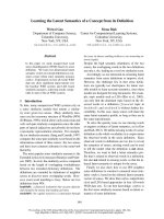
Section 3.3: Feature potency quantization
Feature potency
Section 3.4: Condensed feature construction
F
N (e.g., N=100M)
Original feature set
Section 3.1: Feature potency estimation
Features mapped into this area will be zeroed
by the effect of C
C
0
-C
Section 3.2: Feature potency discounting
Feature potency
ܸ′
஽
݂
௡
0
Feature potency
ܸ
஽
݂
௡
ܸ
∗
஽
݂
௡

( Integer Space N )
Condensed feature set
H
Each condensed feature is represented as a set
of features in the original feature set F.
-1/δ
1/δ
3/δ
φ
-2/δ
M (e.g., M=1K)
The potencies are also utilized as
an (M+1)-th condensed feature
H
ݑ
௡
(Quantized feature potency)
Features mapped into zero are discarded and
never mapped into any condensed features
Figure 1: Outline of our method to construct a condensed
feature set.
¯r(x) =
X
y∈Y(x)
r(x, y)/|Y(x)|.
V
+
D
(f
n

) =
X
x∈D
f
n
(x,
ˆ
y)(r(x,
ˆ
y) − ¯r(x))
V
−
D
(f
n
) = −
X
x∈D
X
y∈Y(x)\
ˆ
y
f
n
(x, y)(r(x, y) − ¯r(x))
R
n
=
X
x∈D

X
y∈Y(x)
r(x, y)f
n
(x, y), A
n
=
X
x∈D
¯r (x)
X
y∈Y(x)
f
n
(x, y)
Figure 2: Notations used in this paper.
terized as a set of features in F, that is, h
m
= S
m
where S
m
⊆ F. We assume that each original fea-
ture f
n
∈F maps, at most, to one condensed feature
h
m
. This assumption prevents two condensed fea-
tures from containing the same original feature, and

some original features from not being mapped to any
condensed feature. Namely, S
m
∩ S
m

=∅ for all m
and m

, where m=m

, and
∪
M
m=1
S
m
⊆F hold.
The value of each condensed feature is calcu-
lated by summing the values of the original fea-
tures assigned to it. Formally, let X and Y repre-
sent the sets of all possible inputs and outputs of
a target task, respectively. Let x ∈ X be an in-
put, and y ∈ Y(x) be an output, where Y(x) ⊆ Y
represents the set of possible outputs given x. We
write the n-th feature function of the original fea-
tures, whose value is determined by x and y, as
f
n
(x, y), where n ∈ {1, . . . , N }. Similarly, we

write the m-th feature function of the condensed fea-
tures as h
m
(x, y), where m∈{1, . . . , M }. We state
that the value of h
m
(x, y) is calculated as follows:
h
m
(x, y)=
∑
f
n
∈S
m
f
n
(x, y).
3 Learning COFERs
The remaining part of our method consists of the
way to map the original features into the condensed
features. For this purpose, we define the feature po-
tency, which is evaluated by employing an existing
supervised model with unsupervised data sets. Fig-
ure 1 shows a brief sketch of the process to construct
the condensed features described in this section.
3.1 Self-taught-style feature potency estimation
We assume that we have a model trained by super-
vised learning, which we call the ‘base supervised
model’, and the original feature set F that is used

in the base supervised model. We consider a case
where the base supervised model is a (log-)linear
model, and use the following equation to select the
best output
ˆ
y given x:
ˆ
y = arg max
y∈Y(x)
∑
N
n=1
w
n
f
n
(x, y),
(1)
where w
n
is a model parameter (or weight) of f
n
.
Linear models are currently the most widely-used
models and are employed in many NLP systems.
To simplify the explanation, we define function
r(x, y), where r(x, y) returns 1 if y =
ˆ
y is obtained
from the base supervised model given x, and 0 oth-

erwise. Let ¯r(x) represent the average of r(x, y) in
x (see Figure 2 for details). We also define V
+
D
(f
n
)
and V
−
D
(f
n
) as shown in Figure 2 where D repre-
sents the unsupervised data set. V
+
D
(f
n
) measures
the positive correlation with the best output
ˆ
y given
by the base supervised model since this is the sum-
mation of all the (weighted) feature values used in
the estimation of the one best output
ˆ
y over all x in
the unsupervised data D. Similarly, V
−
D

(f
n
) mea-
sures the negative correlation with
ˆ
y. Next, we de-
fine V
D
(f
n
) as the feature potency of f
n
: V
D
(f
n
) =
V
+
D
(f
n
) − V
−
D
(f
n
).
An intuitive explanation of V
D

(f
n
) is as follows;
if |V
D
(f
n
)| is large, the distribution of f
n
has either
a large positive or negative correlation with the best
output
ˆ
y given by the base supervised model. This
implies that f
n
is an informative and potent feature
in the model. Then, the distribution of f
n
has very
small (or no) correlation to determine
ˆ
y if |V
D
(f
n
)|
is zero or near zero. In this case, f
n
can be evaluated

as an uninformative feature in the model. From this
perspective, we treat V
D
(f
n
) as a measure of feature
potency in terms of the base supervised model.
The essence of this idea, evaluating features
against each other on a certain model, is widely
used in the context of semi-supervised learning,
i.e., (Ando and Zhang, 2005; Suzuki and Isozaki,
637
2008; Druck and McCallum, 2010). Our method
is rough and a much simpler framework for imple-
menting this fundamental idea of semi-supervised
learning developed for NLP tasks. We create a
simple framework to achieve improved flexibility,
extendability, and applicability. In fact, we apply
the framework by incorporating a feature merging
and elimination architecture to obtain effective con-
densed feature sets for supervised learning.
3.2 Feature potency discounting
To discount low potency values, we redefine feature
potency as V

D
(f
n
) instead of V
D

(f
n
) as follows:
V

D
(f
n
) =



log [R
n
+C]−log[A
n
] if R
n
−A
n
<−C
0 if − C ≤R
n
−A
n
≤C
log [R
n
−C]−log[A
n

] if C < R
n
−A
n
where R
n
and A
n
are defined in Figure 2. Note
that V
D
(f
n
) = V
+
D
(f
n
) − V
−
D
(f
n
) = R
n
− A
n
.
The difference from V
D

(f
n
) is that we cast it in the
log-domain and introduce a non-negative constant
C. The introduction of C is inspired by the L
1
-
regularization technique used in supervised learning
algorithms such as (Duchi and Singer, 2009; Tsu-
ruoka et al., 2009). C controls how much we dis-
count V
D
(f
n
) toward zero, and is given by the user.
3.3 Feature potency quantization
We define V
∗
D
(f
n
) as V
∗
D
(f
n
) = δV

D
(f

n
) if
V

D
(f
n
) > 0 and V
∗
D
(f
n
) = δV

D
(f
n
) otherwise,
where δ is a positive user-specified constant. Note
that V
∗
D
(f
n
) always becomes an integer, that is,
V
∗
D
(f
n

) ∈ N where N = {. . . , −2, −1, 0, 1, 2, . . .}.
This calculation can be seen as mapping each fea-
ture into a discrete (integer) space with respect to
V

D
(f
n
). δ controls the range of V

D
(f
n
) mapping
into the same integer.
3.4 Condensed feature construction
Suppose we have M different quantized feature po-
tency values in V
∗
D
(f
n
) for all n, which we rewrite
as {u
m
}
M
m=1
. Then, we define S
m

as a set of f
n
whose quantized feature potency value is u
m
. As
described in Section 2, we define the m-th con-
densed feature h
m
(x, y) as the summation of all
the original features f
n
assigned to S
m
. That is,
h
m
(x, y) =
∑
f
n
∈S
m
f
n
(x, y). This feature fusion
process is intuitive since it is acceptable if features
with the same (similar) feature potency are given the
same weight by supervised learning since they have
the same potency with regard to determining
ˆ

y. δ
determines the number of condensed features to be
made; the number of condensed features becomes
large if δ is large. Obviously, the upper bound of
the number of condensed features is the number of
original features.
To exclude possibly unnecessary original features
from the condensed features, we discard feature f
n
for all n if u
n
= 0. This is reasonable since, as de-
scribed in Section 3.1, a feature has small (or no)
effect in achieving the best output decision in the
base supervised model if its potency is near 0. C in-
troduced in Section 3.2 mainly influences how many
original features are discarded.
Additionally, we also utilize the ‘quantized’ fea-
ture potency values themselves as a new feature.
The reason behind is that they are also very infor-
mative for supervised learning. Their use is impor-
tant to further boost the performance gain offered
by our method. For this purpose, we define φ(x, y)
as φ(x, y) =
∑
M
m=1
(u
m
/δ)h

m
(x, y). We then
use φ(x, y) as the (M + 1)-th feature of our con-
densed feature set. As a result, the condensed fea-
ture set obtained with our method is represented as
H = {h
1
(x, y), . . . , h
M
(x, y), φ(x, y)}.
Note that the calculation cost of φ(x, y) is negli-
gible. We can calculate the linear discriminant func-
tion g(x, y) as: g(x, y) =
∑
M
m=1
w
m
h
m
(x, y) +
w
M+1
φ(x, y) =
∑
M
m=1
w

m

h
m
(x, y), where w

m
=
(w
m
+ w
M+1
u
m
/δ). We emphasize that once
{w
m
}
M+1
m=1
are determined by supervised learning,
we can calculate w

m
in a preliminary step before
the test phase. Thus, our method also takes the form
of a linear model. The number of features for our
method is essentially M even if we add φ.
3.5 Application to Structured Prediction Tasks
We modify our method to better suit structured pre-
diction problems in terms of calculation cost. For a
structured prediction problem, it is usual to decom-

pose or factorize output structure y into a set of lo-
cal sub-structures z to reduce the calculation cost
and to cope with the sparsity of the output space
Y. This factorization can be accomplished by re-
stricting features that are extracted only from the in-
formation within decomposed local sub-structure z
638
and given input x. We write z ∈ y when the lo-
cal sub-structure z is a part of output y, assuming
that output y is constructed by a set of local sub-
structures. Then formally, the n-th feature is written
as f
n
(x, z), and f
n
(x, y) =
∑
z∈y
f
n
(x, z) holds.
Similarly, we introduce r(x, z) , where r(x , z) = 1
if z ∈
ˆ
y, and r(x, z) = 0 otherwise, namely z /∈
ˆ
y.
We define Z(x) as the set of all local sub-
structures possibly generated for all y in Y(x).
Z(x) can be enumerated easily, unless we use typi-

cal first- or second-order factorization models by the
restriction of efficient decoding algorithms, which is
the typical case for many NLP tasks such as named
entity recognition and dependency parsing.
Finally, we replace all Y(x) with Z(x), and use
f
n
(x, z) and r(x, z) instead of f
n
(x, y) and r(x, y),
respectively, in R
n
and A
n
. When we use these sub-
stitutions, there is no need to incorporate an efficient
algorithm such as dynamic programming into our
method. This means that our feature potency esti-
mation can be applied to the structured prediction
problem at low cost.
3.6 Efficient feature potency computation
Our feature potency estimation described in Section
3.1 to 3.3 is highly suitable for implementation in
the MapReduce framework (Dean and Ghemawat,
2008), which is a modern distributed parallel com-
puting framework. This is because R
n
and A
n
can

be calculated by the summation of a data-wise cal-
culation (map phase), and V
∗
D
(f
n
) can be calculated
independently by each feature (reduce phase). We
emphasize that our feature potency estimation can
be performed in a ‘single’ map-reduce process.
4 Experiments
We conducted experiments on two different NLP
tasks, namely NER and dependency parsing. To fa-
cilitate comparisons with the performance of previ-
ous methods, we adopted the experimental settings
used to examine high-performance semi-supervised
NLP systems; i.e., NER (Ando and Zhang, 2005;
Suzuki and Isozaki, 2008) and dependency pars-
ing (Koo et al., 2008; Chen et al., 2009; Suzuki
et al., 2009). For the supervised datasets, we used
CoNLL’03 (Tjong Kim Sang and De Meulder, 2003)
shared task data for NER, and the Penn Treebank III
(PTB) corpus (Marcus et al., 1994) for dependency
parsing. We prepared a total of 3.72 billion token
text data as unsupervised data following the instruc-
tions given in (Suzuki et al., 2009).
4.1 Comparative Methods
We mainly compare the effectiveness of COFER
with that of CWR derived by the Brown algorithm.
The iCWR approach yields the state-of-the-art re-

sults with both dependency parsing data derived
from PTB-III (Koo et al., 2008), and the CoNLL’03
shared task data (Turian et al., 2010). By compar-
ing COFER with iCWR we can clarify its effective-
ness in terms of providing better features for super-
vised learning. We use the term active features to
refer to features whose corresponding model param-
eter is non-zero after supervised learning. It is well-
known that we can discard non-active features from
the trained model without any loss after finishing su-
pervised learning. Finally, we compared the perfor-
mance in terms of the number of active features in
the model given by supervised learning. We note
here that the number of active features for COFER
is the number of features h
m
if w

m
= 0, which is
not w
m
= 0 for a fair comparison.
Unlike COFER, iCWR does not have any archi-
tecture to winnow the original feature set used in
supervised learning. For a fair comparison, we
prepared L
1
-regularized supervised learning algo-
rithms, which try to reduce the non-zero parameters

in a model. Specifically, we utilized L
1
-regularized
CRF (L1CRF) optimized by OWL-QN (Andrew
and Gao, 2007) for NER, and the online struc-
tured output learning version of FOBOS (Duchi
and Singer, 2009; Tsuruoka et al., 2009) with L
1
-
regularization (ostL1FOBOS) for dependency pars-
ing. In addition, we also examined L
2
regular-
ized CRF (Lafferty et al., 2001) optimized by L-
BFGS (Liu and Nocedal, 1989) ( L2CRF) for NER,
and the online structured output learning version of
the Passive-Aggressive algorithm (ostPA) (Cram-
mer et al., 2006) for dependency parsing to illus-
trate the baseline performance regardless of the ac-
tive feature number.
4.2 Settings for COFER
We utilized baseline supervised learning mod-
els as the base supervised models of COFER.
639
86.0
88.0
90.0
92.0
94.0
96.0

1.0E+01 1.0E+03 1.0E+05 1.0E+07 1.0E+09
iCWR+COFER: L2CRF iCWR+COFER: L1CRF
COFER: L2CRF COFER: L1CRF
iCWR: L2CRF iCWR: L1CRF
Sup.L2CRF Sup.L1CRF
F
-
score
# of active features [log-scale]
δ=1e+01
δ=1e+02
δ=1e+04
δ=1e+00
proposed
90.0
91.0
92.0
93.0
94.0
95.0
1.E+02 1.E+04 1.E+06 1.E+08
iCWR+COFER: ostPA iCWR+COFER: ostL1FOBOS
COFER: ostPA COFER: ostL1FOBOS
iCWR: ostPA iCWR: ostL1FOBOS
Sup.ostPA Sup.ostL1FOBOS
# of active features [log-scale]
Unlabeled Attachment Score
δ
=1e+00
δ

=1e+05
δ
=1e+01
δ
=1e+03
proposed
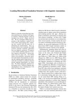
(a) NER (F-score) (b) dep. parsing (UAS)
Figure 3: Performance vs. size of active features in the
trained model on the development sets
In addition, we also report the results when we
treat iCWR as COFER’s base supervised mod-
els (iCWR+COFER). This is a very natural and
straightforward approach to combining these two.
We generally handle several different types of fea-
tures such as words, part-of-speech tags, word sur-
face forms, and their combinations. Suppose we
have K different feature types, which are often de-
fined by feature templates, i.e., (Suzuki and Isozaki,
2008; Lin and Wu, 2009). In our experiments, we re-
strict the merging of features during the condensed
feature construction process if and only if the fea-
tures are the same feature type. As a result, COFER
essentially consists of K different condensed feature
sets. The numbers of feature types K were 79 and 30
for our NER and dependency parsing experiments,
respectively. We note that this kind of feature par-
tition by their types is widely used in the context of
semi-supervised learning (Ando and Zhang, 2005;
Suzuki and Isozaki, 2008).
4.3 Results and Discussion

Figure 3 displays the performance on the develop-
ment set with respect to the number of active fea-
tures in the trained models given by each supervised
learning algorithm. In both NER and dependency
parsing experiments, COFER significantly outper-
formed iCWR. Moreover, COFER was surprisingly
robust in relation to the number of active features
in the model. These results reveal that COFER pro-
vides effective feature sets for certain NLP tasks.
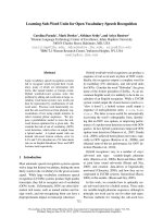
We summarize the noteworthy results in Figure 3,
and also the performance of recent top-line systems
for NER and dependency parsing in Table 1. Over-
all, COFER matches the results of top-line semi-
NER system dev. test #.USD #.AF
Sup.L1CRF 90.40 85.08 0 0.57M
iCWR: L1CRF 93.33 89.99 3,720M 0.62M
COFER: L1CRF (δ = 1e + 00) 93.42 88.81 3,720M 359
(δ = 1e + 04) 93.60 89.22 3,720M 2.46M
iCWR+COFER: (δ = 1e + 00) 94.39 90.72 3,720M 344
L1CRF (δ = 1e + 04) 94.91 91.02 3,720M 5.94M
(Ando and Zhang, 2005) 93.15 89.31 27M N/A
(Suzuki and Isozaki, 2008) 94.48 89.92 1,000M N/A
(Ratinov and Roth, 2009) 93.50 90.57 N/A N/A
(Turian et al., 2010) 93.95 90.36 37M N/A
(Lin and Wu, 2009) N/A 90.90 700,000M N/A
Dependency parser dev. test #.USD #.AF
ostL1FOBOS 93.15 92.82 0 6.80M
iCWR: ostL1FOBOS 93.69 93.49 3,720M 9.67M
COFER:ostL1FOBOS (δ = 1e + 03) 93.53 93.23 3,720M 20.7K
(δ = 1e + 05) 93.91 93.71 3,720M 3.23M

iCWR+COFER: (δ = 1e + 03) 93.93 93.55 3,720M 12.5K
ostL1FOBOS (δ = 1e + 05) 94.33 94.22 3,720M 5.77M
(Koo and Collins, 2010) 93.49 93.04 0 N/A
(Martins et al., 2010) N/A 93.26 0 55.25M
(Koo et al., 2008) 93.30 93.16 43M N/A
(Chen et al., 2009) N/A 93.16 43M N/A
(Suzuki et al., 2009) 94.13 93.79 3,720M N/A
Table 1: Comparison with previous top-line systems on
test data. (#.USD: unsupervised data size. #.AF: the size
of active features in the trained model.)
supervised learning systems even though it uses far
fewer active features.
In addition, the combination of iCWR+COFER
significantly outperformed the current best results
by achieving a 0.12 point gain from 90.90 to 91.02
for NER, and a 0.43 point gain from 93.79 to 94.22
for dependency parsing, with only 5.94M and 5.77M
features, respectively.
5 Conclusion
This paper introduced the idea of condensed feature
representations (COFER) as a simple and general
framework that can enhance the performance of ex-
isting supervised NLP systems. We also proposed
a method that efficiently constructs condensed fea-
ture sets through discrete feature potency estima-
tion over unsupervised data. We demonstrated that
COFER based on our feature potency estimation can
offer informative dense and low-dimensional feature
spaces for supervised learning, which is theoreti-
cally preferable to the sparse and high-dimensional

feature spaces often used in many NLP tasks. Exist-
ing NLP systems can be made more compact with
higher performance by retraining their models with
our condensed features.
640
References
Rie Kubota Ando and Tong Zhang. 2005. A High-
Performance Semi-Supervised Learning Method for
Text Chunking. In Proceedings of 43rd Annual Meet-
ing of the Association for Computational Linguistics,
pages 1–9.
Galen Andrew and Jianfeng Gao. 2007. Scalable
Training of L1-regularized Log-linear Models. In
Zoubin Ghahramani, editor, Proceedings of the 24th
Annual International Conference on Machine Learn-
ing (ICML 2007), pages 33–40. Omnipress.
Wenliang Chen, Jun’ichi Kazama, Kiyotaka Uchimoto,
and Kentaro Torisawa. 2009. Improving Dependency
Parsing with Subtrees from Auto-Parsed Data. In Pro-
ceedings of the 2009 Conference on Empirical Meth-
ods in Natural Language Processing, pages 570–579.
Koby Crammer, Ofer Dekel, Joseph Keshet, Shai Shalev-
Shwartz, and Yoram Singer. 2006. Online Passive-
Aggressive Algorithms. Journal of Machine Learning
Research, 7:551–585.
Jeffrey Dean and Sanjay Ghemawat. 2008. MapReduce:
Simplified Data Processing on Large Clusters. Com-
mun. ACM, 51(1):107–113.
Gregory Druck and Andrew McCallum. 2010. High-
Performance Semi-Supervised Learning using Dis-

criminatively Constrained Generative Models. In Pro-
ceedings of the International Conference on Machine
Learning (ICML 2010), pages 319–326.
John Duchi and Yoram Singer. 2009. Efficient On-
line and Batch Learning Using Forward Backward
Splitting. Journal of Machine Learning Research,
10:2899–2934.
Terry Koo and Michael Collins. 2010. Efficient Third-
Order Dependency Parsers. In Proceedings of the 48th
Annual Meeting of the Association for Computational
Linguistics, pages 1–11.
Terry Koo, Xavier Carreras, and Michael Collins. 2008.
Simple Semi-supervised Dependency Parsing. In Pro-
ceedings of ACL-08: HLT, pages 595–603.
John Lafferty, Andrew McCallum, and Fernando Pereira.
2001. Conditional Random Fields: Probabilistic Mod-
els for Segmenting and Labeling Sequence Data. In
Proceedings of the International Conference on Ma-
chine Learning (ICML 2001), pages 282–289.
Dekang Lin and Xiaoyun Wu. 2009. Phrase Cluster-
ing for Discriminative Learning. In Proceedings of
the Joint Conference of the 47th Annual Meeting of
the ACL and the 4th International Joint Conference
on Natural Language Processing of the AFNLP, pages
1030–1038.
Dong C. Liu and Jorge Nocedal. 1989. On the Limited
Memory BFGS Method for Large Scale Optimization.
Math. Programming, Ser. B, 45(3):503–528.
Mitchell P. Marcus, Beatrice Santorini, and Mary Ann
Marcinkiewicz. 1994. Building a Large Annotated

Corpus of English: The Penn Treebank. Computa-
tional Linguistics, 19(2):313–330.
Andre Martins, Noah Smith, Eric Xing, Pedro Aguiar,
and Mario Figueiredo. 2010. Turbo Parsers: Depen-
dency Parsing by Approximate Variational Inference.
In Proceedings of the 2010 Conference on Empirical
Methods in Natural Language Processing, pages 34–
44.
Lev Ratinov and Dan Roth. 2009. Design Challenges
and Misconceptions in Named Entity Recognition. In
Proceedings of the Thirteenth Conference on Compu-
tational Natural Language Learning (CoNLL-2009),
pages 147–155.
Jun Suzuki and Hideki Isozaki. 2008. Semi-supervised
Sequential Labeling and Segmentation Using Giga-
Word Scale Unlabeled Data. In Proceedings of ACL-
08: HLT, pages 665–673.
Jun Suzuki, Hideki Isozaki, Xavier Carreras, and Michael
Collins. 2009. An Empirical Study of Semi-
supervised Structured Conditional Models for Depen-
dency Parsing. In Proceedings of the 2009 Conference
on Empirical Methods in Natural Language Process-
ing, pages 551–560.
Erik Tjong Kim Sang and Fien De Meulder. 2003. Intro-
duction to the CoNLL-2003 Shared Task: Language-
Independent Named Entity Recognition. In Proceed-
ings of CoNLL-2003, pages 142–147.
Yoshimasa Tsuruoka, Jun’ichi Tsujii, and Sophia Ana-
niadou. 2009. Stochastic Gradient Descent Training
for L1-regularized Log-linear Models with Cumula-

tive Penalty. In Proceedings of the Joint Conference
of the 47th Annual Meeting of the ACL and the 4th
International Joint Conference on Natural Language
Processing of the AFNLP, pages 477–485.
Joseph Turian, Lev-Arie Ratinov, and Yoshua Bengio.
2010. Word Representations: A Simple and General
Method for Semi-Supervised Learning. In Proceed-
ings of the 48th Annual Meeting of the Association for
Computational Linguistics, pages 384–394.
641