Báo cáo khoa học: "Advances in Discriminative Parsing" potx
Bạn đang xem bản rút gọn của tài liệu. Xem và tải ngay bản đầy đủ của tài liệu tại đây (98.05 KB, 8 trang )
Proceedings of the 21st International Conference on Computational Linguistics and 44th Annual Meeting of the ACL, pages 873–880,
Sydney, July 2006.
c
2006 Association for Computational Linguistics
Advances in Discriminative Parsing
Joseph Turian and I. Dan Melamed
{lastname}@cs.nyu.edu
Computer Science Department
New York University
New York, New York 10003
Abstract
The present work advances the accu-
racy and training speed of discrimina-
tive parsing. Our discriminative parsing
method has no generative component, yet
surpasses a generative baseline on con-
stituent parsing, and does so with mini-
mal linguistic cleverness. Our model can
incorporate arbitrary features of the in-
put and parse state, and performs fea-
ture selection incrementally over an ex-
ponential feature space during training.
We demonstrate the flexibility of our ap-
proach by testing it with several pars-
ing strategies and various feature sets.
Our implementation is freely available at:
/>1 Introduction
Discriminative machine learning methods have
improved accuracy on many NLP tasks, including
POS-tagging, shallow parsing, relation extraction,
and machine translation. Some advances have also
been made on full syntactic constituent parsing.
Successful discriminative parsers have relied on
generative models to reduce training time and
raise accuracy above generative baselines (Collins
& Roark, 2004; Henderson, 2004; Taskar et al.,
2004). However, relying on information from a
generative model might prevent these approaches
from realizing the accuracy gains achieved by dis-
criminative methods on other NLP tasks. Another
problem is training speed: Discriminative parsers
are notoriously slow to train.
In the present work, we make progress towards
overcoming these obstacles. We propose a flexi-
ble, end-to-end discriminative method for training
parsers, demonstrating techniques that might also
be useful for other structured prediction problems.
The proposed method does model selection with-
out ad-hoc smoothing or frequency-based feature
cutoffs. It requires no heuristics or human effort
to optimize the single important hyper-parameter.
The training regime can use all available informa-
tion from the entire parse history. The learning al-
gorithm projects the hand-provided features into a
compound feature space and performs incremen-
tal feature selection over this large feature space.
The resulting parser achieves higher accuracy than
a generative baseline, despite not using a genera-
tive model as a feature.
Section 2 describes the parsing algorithm. Sec-
tion 3 presents the learning method. Section 4
presents experiments with discriminative parsers
built using these methods. Section 5 compares our
approach to related work.
2 Parsing Algorithm
The following terms will help to explain our work.
A span is a range over contiguous words in the in-
put. Spans cross if they overlap but neither con-
tains the other. An item is a (span, label) pair. A
state is a partial parse, i.e. a set of items, none
of whose spans may cross. A parse inference is
a (state, item) pair, i.e. a state and an item to be
added to it. The frontier of a state consists of the
items with no parents yet. The children of a candi-
date inference are the frontier items below the item
to be inferred, and the head of a candidate infer-
ence is the child item chosen by English head rules
(Collins, 1999, pp. 238–240). A parse path is a
sequence of parse inferences. For some input sen-
tence and training parse tree, a state is correct if
the parser can infer zero or more additional items
to obtain the training parse tree, and an inference
873
is correct if it leads to a correct state.
Given input sentence s, the parser searches for
parse ˆp out of the possible parses P(s):
ˆp = arg min
p∈P(s)
C
Θ
(p) (1)
where C
Θ
(p) is the cost of parse p under model Θ:
C
Θ
(p) =
i∈p
c
Θ
(i) (2)
Section 3.1 describes how to compute c
Θ
(i). Be-
cause c
Θ
(i) ∈ R
+
, the cost of a partial parse mono-
tonically increases as we add items to it.
The parsing algorithm considers a succession
of states. The initial state contains terminal items,
whose labels are the POS tags given by the tagger
of Ratnaparkhi (1996). Each time we pop a state
from the agenda, c
Θ
computes the costs for the
candidate bottom-up inferences generated from
that state. Each candidate inference results in a
successor state to be placed on the agenda.
The cost function c
Θ
can consider arbitrary
properties of the input and parse state. We are not
aware of any tractable solution to Equation 1, such
as dynamic programming. Therefore, the parser
finds ˆp using a variant of uniform-cost search.
The parser implements the search using an agenda
that stores entire states instead of single items.
Each time a state is popped from the agenda, the
parser uses depth-first search starting from the
state that was popped until it (greedily) finds a
complete parse. In preliminary experiments, this
search strategy was faster than standard uniform-
cost search (Russell & Norvig, 1995).
3 Training Method
3.1 General Setting
Our training set I consists of candidate inferences
from the parse trees in the training data. From
each training inference i ∈ I we generate the tuple
X(i), y(i), b(i). X(i) is a feature vector describing
i, with each element in {0, 1}. We will use X
f
(i) to
refer to the element of X(i) that pertains to feature
f. y(i) = +1 if i is correct, and y(i) = −1 if not.
Some training examples might be more important
than others, so each is given a bias b(i) ∈ R
+
, as
detailed in Section 3.3.
The goal during training is to induce a hypothe-
sis h
Θ
(i), which is a real-valued inference scoring
function. In the present work, h
Θ
is a linear model
parameterized by a real vector Θ, which has one
entry for each feature f:
h
Θ
(i) = Θ · X(i) =
f
Θ
f
· X
f
(i) (3)
The sign of h
Θ
(i) predicts the y-value of i and the
magnitude gives the confidence in this prediction.
The training procedure optimizes Θ to minimize
the expected risk R
Θ
over training set I. R
Θ
is the
objective function, a combination of loss function
L
Θ
and regularization term Ω
Θ
:
R
Θ
(I) = L
Θ
(I) + Ω
Θ
(4)
The loss of the inference set decomposes into the
loss of individual inferences:
L
Θ
(I) =
i∈I
l
Θ
(i) (5)
In principle, l
Θ
can be any loss function, but in the
present work we use the log-loss (Collins et al.,
2002):
l
Θ
(i) = b(i) · ln(1 + exp(−µ
Θ
(i))) (6)
and µ
Θ
(i) is the margin of inference i:
µ
Θ
(i) = y(i) · h
Θ
(i) (7)
Inference cost c
Θ
(i) in Equation 2 is l
Θ
(i) com-
puted using y(i) = +1 and b(i) = 1, i.e.:
c
Θ
(i) = ln(1 + exp(−h
Θ
(i))) (8)
Ω
Θ
in Equation 4 is a regularizer, which penal-
izes complex models to reduce overfitting and gen-
eralization error. We use the
1
penalty:
Ω
Θ
=
f
λ · |Θ
f
| (9)
where λ is a parameter that controls the strength
of the regularizer. This choice of objective R
Θ
is
motivated by Ng (2004), who suggests that, given
a learning setting where the number of irrelevant
features is exponential in the number of train-
ing examples, we can nonetheless learn effectively
by building decision trees to minimize the
1
-
regularized log-loss. On the other hand, Ng (2004)
suggests that most of the learning algorithms com-
monly used by discriminative parsers will overfit
when exponentially many irrelevant features are
present.
1
Learning over an exponential feature space is
the very setting we have in mind. A priori, we de-
fine only a set A of simple atomic features (given
1
including the following learning algorithms:
• unregularized logistic regression
• logistic regression with an
2
penalty (i.e. a Gaussian prior)
• SVMs using most kernels
• multilayer neural nets trained by backpropagation
• the perceptron algorithm
874
in Section 4). The learner then induces compound
features, each of which is a conjunction of possi-
bly negated atomic features. Each atomic feature
can have one of three values (yes/no/don’t care),
so the size of the compound feature space is 3
|A|
,
exponential in the number of atomic features. It
was also exponential in the number of training ex-
amples in our experiments (|A| ≈ |I|).
3.2 Boosting
1
-Regularized Decision Trees
We use an ensemble of confidence-rated decision
trees (Schapire & Singer, 1999) to represent h
Θ
.
2
The path from the root to each node n in a decision
tree corresponds to some compound feature f, and
we write ϕ(n) = f. To score an inference i using
a decision tree, we percolate the inference’s fea-
tures X(i) down to a leaf n and return confidence
Θ
ϕ(n)
. An inference i percolates down to node n iff
X
ϕ(n)
= 1. Each leaf node n keeps track of the pa-
rameter value Θ
ϕ(n)
.
3
The score h
Θ
(i) given to an
inference i by the whole ensemble is the sum of the
confidences returned by the trees in the ensemble.
Listing 1 Outline of training algorithm.
1: procedure T(I)
2: ensemble ← ∅
3: λ ← ∞
4: while dev set accuracy is increasing do
5: t ← tree with one (root) node
6: while the root node cannot be split do
7: decay
1
parameter λ
8: while some leaf in t can be split do
9: split the leaf to maximize gain
10: percolate every i ∈ I to a leaf node
11: for each leaf n in t do
12: update Θ
ϕ(n)
to minimize R
Θ
13: append t to ensemble
Listing 1 presents our training algorithm. At
the beginning of training, the ensemble is empty,
Θ = 0, and the
1
parameter λ is set to ∞ (Steps 1.2
and 1.3). We train until the objective cannot be fur-
ther reduced for the current choice of λ. We then
determine the accuracy of the parser on a held-out
development set using the previous λ value (be-
fore it was decreased), and stop training when this
2
Turian and Melamed (2005) reported that decision trees
applied to parsing have higher accuracy and training speed
than decision stumps, so we build full decision trees rather
than stumps.
3
Any given compound feature can appear in more than one
tree, but each leaf node has a distinct confidence value. For
simplicity, we ignore this possibility in our discussion.
accuracy reaches a plateau (Step 1.4). Otherwise,
we relax the regularization penalty by decreasing
λ (Steps 1.6 and 1.7) and continue training. In this
way, instead of choosing the best λ heuristically,
we can optimize it during a single training run
(Turian & Melamed, 2005).
Each training iteration (Steps 1.5–1.13) has sev-
eral steps. First, we choose some compound fea-
tures that have high magnitude gradient with re-
spect to the objective function. We do this by
building a new decision tree, whose leaves rep-
resent the chosen compound features (Steps 1.5–
1.9). Second, we confidence-rate each leaf to min-
imize the objective over the examples that per-
colate down to that leaf (Steps 1.10–1.12). Fi-
nally, we append the decision tree to the ensem-
ble and update parameter vector Θ accordingly
(Step 1.13). In this manner, compound feature se-
lection is performed incrementally during train-
ing, as opposed to a priori.
Our strategy minimizing the objective R
Θ
(I)
(Equation 4) is a variant of steepest descent
(Perkins et al., 2003). To compute the gradient of
the unpenalized loss L
Θ
with respect to the param-
eter Θ
f
of feature f, we have:
∂L
Θ
(I)
∂Θ
f
=
i∈I
∂l
Θ
(i)
∂µ
Θ
(i)
·
∂µ
Θ
(i)
∂Θ
f
(10)
where:
∂µ
Θ
(i)
∂Θ
f
= y(i) · X
f
(i) (11)
Using Equation 6, we define the weight of an ex-
ample i under the current model as the rate at
which loss decreases as the margin of i increases:
w
Θ
(i) = −
∂l
Θ
(i)
∂µ
Θ
(i)
= b(i) ·
1
1 + exp(µ
Θ
(i))
(12)
Recall that X
f
(i) is either 0 or 1. Combining Equa-
tions 10–12 gives:
∂L
Θ
(I)
∂Θ
f
= −
i∈I
X
f
(i)=1
y(i) · w
Θ
(i) (13)
We define the gain of feature f as:
G
Θ
(I; f) = max
0,
∂L
Θ
(I)
∂Θ
f
− λ
(14)
Equation 14 has this form because the gradient of
the penalty term is undefined at Θ
f
= 0. This dis-
continuity is why
1
regularization tends to pro-
duce sparse models. If G
Θ
(I; f) = 0, then the ob-
jective R
Θ
(I) is at its minimum with respect to pa-
rameter Θ
f
. Otherwise, G
Θ
(I; f) is the magnitude
875
of the gradient of the objective as we adjust Θ
f
in
the appropriate direction.
To build each decision tree, we begin with a root
node. The root node corresponds to a dummy “al-
ways true” feature. We recursively split nodes by
choosing a splitting feature that will allow us to in-
crease the gain. Node n with corresponding com-
pound feature ϕ(n) = f can be split by atomic fea-
ture a if:
G
Θ
(I; f ∧ a) + G
Θ
(I; f ∧ ¬a) > G
Θ
(I; f) (15)
If no atomic feature satisfies the splitting crite-
rion in Equation 15, then n becomes a leaf node
of the decision tree and Θ
ϕ(n)
becomes one of the
values to be optimized during the parameter up-
date step. Otherwise, we choose atomic feature ˆa
to split node n:
ˆa = argmax
a∈A
(
G
Θ
(I; f ∧ a) + G
Θ
(I; f ∧ ¬a)
)
(16)
This split creates child nodes n
1
and n
2
, with
ϕ(n
1
) = f ∧ ˆa and ϕ(n
2
) = f ∧ ¬ˆa.
Parameter update is done sequentially on only
the most recently added compound features, which
correspond to the leaves of the new decision tree.
After the entire tree is built, we percolate exam-
ples down to their appropriate leaf nodes. We then
choose for each leaf node n the parameter Θ
ϕ(n)
that minimizes the objective over the examples in
that leaf. A convenient property of decision trees
is that the leaves’ compound features are mutually
exclusive. Their parameters can be directly opti-
mized independently of each other using a line
search over the objective.
3.3 The Training Set
We choose a single correct path from each training
parse tree, and the training examples correspond to
all candidate inferences considered in every state
along this path.
4
In the deterministic setting there
is only one correct path, so example generation
is identical to that of Sagae and Lavie (2005). If
parsing proceeds non-deterministically then there
might be multiple paths that lead to the same final
parse, so we choose one randomly. This method
of generating training examples does not require a
working parser and can be run prior to any train-
ing. The disadvantage of this approach is that it
minimizes the error of the parser at correct states
only. It does not account for compounded error or
4
Nearly all of the examples generated are negative (y = −1).
teach the parser to recover from mistakes grace-
fully.
Turian and Melamed (2005) observed that uni-
form example biases b(i) produced lower accuracy
as training progressed, because the induced clas-
sifiers minimized the error per example. To min-
imize the error per state, we assign every train-
ing state equal value and share half the value uni-
formly among the negative examples for the ex-
amples generated from that state and the other half
uniformly among the positive examples.
We parallelize training by inducing 26 label
classifiers (one for each non-terminal label in the
Penn Treebank). Parallelization might not uni-
formly reduce training time because different la-
bel classifiers train at different rates. However, par-
allelization uniformly reduces memory usage be-
cause each label classifier trains only on inferences
whose consequent item has that label.
4 Experiments
Discriminative parsers are notoriously slow to
train. For example, Taskar et al. (2004) took sev-
eral months to train on the ≤ 15 word sentences
in the English Penn Treebank (Dan Klein, p.c.).
The present work makes progress towards faster
discriminative parser training: our slowest classi-
fier took fewer than 5 days to train. Even so, it
would have taken much longer to train on the en-
tire treebank. We follow Taskar et al. (2004) in
training and testing on ≤ 15 word sentences in
the English Penn Treebank (Taylor et al., 2003).
We used sections 02–21 for training, section 22
for development, and section 23 for testing, pre-
processed as per Table 1. We evaluated our parser
using the standard PARSEVAL measures (Black et
al., 1991): labelled precision, labelled recall, and
labelled F-measure (Prec., Rec., and F
1
, respec-
tively), which are based on the number of non-
terminal items in the parser’s output that match
those in the gold-standard parse.
5
As mentioned in Section 2, items are inferred
bottom-up and the parser cannot infer any item
that crosses an item already in the state. Although
there are O(n
2
) possible (span, label) pairs over a
frontier containing n items, we reduce this to the
≈ 5 · n inferences that have at most five children.
6
5
The correctness of a stratified shuffling test has been called
into question (Michael Collins, p.c.), so we are not aware of
any valid significance tests for observed differences in PAR-
SEVAL scores.
6
Only 0.57% of non-terminals in the preprocessed develop-
876
Table 1 Steps for preprocessing the data. Starred steps are performed only when parse trees are available
in the data (e.g. not on test data).
1. * Strip functional tags and trace indices, and remove traces.
2. * Convert PRT to ADVP. (This convention was established by Magerman (1995).)
3. Remove quotation marks (i.e. terminal items tagged ‘‘ or ’’). (Bikel, 2004)
4. * Raise punctuation. (Bikel, 2004)
5. Remove outermost punctuation.
a
6. * Remove unary projections to self (i.e. duplicate items with the same span and label).
7. POS tag the text using the tagger of Ratnaparkhi (1996).
8. Lowercase headwords.
a
As pointed out by an anonymous reviewer of Collins (2003), removing outermost punctuation might discard useful infor-
mation. Collins and Roark (2004) saw a LFMS improvement of 0.8% over their baseline discriminative parser after adding
punctuation features, one of which encoded the sentence-final punctuation.
To ensure the parser does not enter an infinite loop,
no two items in a state can have both the same
span and the same label. Given these restrictions
on candidate inferences, there were roughly 40
million training examples generated in the train-
ing set. These were partitioned among the 26 con-
stituent label classifiers. Building a decision tree
(Steps 1.5–1.9 in Listing 1) using the entire ex-
ample set I can be very expensive. We estimate
loss gradients (Equation 13) using a sample of the
inference set, which gives a 100-fold increase in
training speed (Turian & Melamed, 2006).
Our atomic feature set A contains 300K fea-
tures, each of the form “is there an item in group
J whose label/headword/headtag/headtagclass is
‘X’?”.
7
Possible values of ‘X’ for each predicate
are collected from the training data. For 1 ≤ n ≤ 3,
possible values for J are:
• the first/last n child items
• the first n left/right context items
• the n children items left/right of the head
• the head item.
The left and right context items are the frontier
items to the left and right of the children of the
candidate inference, respectively.
4.1 Different Parsing Strategies
To demonstrate the flexibility of our learn-
ing procedure, we trained three different
parsers: left-to-right (l2r), right-to-left (r2l),
ment set have more than five children.
7
The predicate headtagclass is a supertype of the headtag.
Given our compound features, these arenot strictly necessary,
but they accelerate training. An example is “proper noun,”
which contains the POS tags given to singular and plural
proper nouns. Space constraints prevent enumeration of the
headtagclasses, which are instead provided at the URL given
in the abstract.
Table 2 Results on the development set, training
and testing using only ≤ 15 word sentences.
active
λ features % Rec. % Prec. F
1
l2r 0.040 11.9K 89.86 89.63 89.74
b.u. 0.020 13.7K 89.92 89.84 89.88
r2l 0.014 14.0K 90.66 89.81 90.23
and non-deterministic bottom-up (b.u.). The
non-deterministic parser was allowed to choose
any bottom-up inference. The other two parsers
were deterministic: bottom-up inferences had
to be performed strictly left-to-right or right-
to-left, respectively. We stopped training when
each parser had 15K active features. Figure 1
shows the accuracy of the different runs over the
development set as training progressed. Table 2
gives the PARSEVAL scores of these parsers at
their optimal
1
penalty setting. We found that
the perplexity of the r2l model was low so that,
in 85% of the sentences, its greedy parse was the
optimal one. The l2r parser does poorly because
its decisions were more difficult than those of the
other parsers. If it inferred far-right items, it was
more likely to prevent correct subsequent infer-
ences that were to the left. But if it inferred far-left
items, then it went against the right-branching
tendency of English sentences. The left-to-right
parser would likely improve if we were to use a
left-corner transform (Collins & Roark, 2004).
Parsers in the literature typically choose some
local threshold on the amount of search, such as
a maximum beam width. With an accurate scor-
ing function, restricting the search space using
a fixed beam width might be unnecessary. In-
stead, we imposed a global threshold on explo-
ration of the search space. Specifically, if the
877
Figure 1 F
1
scores on the development set of the
Penn Treebank, using only ≤ 15 word sentences.
The x-axis shows the number of non-zero param-
eters in each parser, summed over all classifiers.
85%
86%
87%
88%
89%
90%
15K10K5K2.5K1.5K
Devel. F-measure
total number of non-zero parameters
right-to-left
left-to-right
bottom up
parser has found some complete parse and has
explored at least 100K states (i.e. scored at least
100K inferences), search stopped prematurely and
the parser would return the (possibly sub-optimal)
current best complete parse. The l2r and r2l
parsers never exceeded this threshold, and al-
ways found the optimal complete parse. However,
the non-deterministic bottom-up parser’s search
was cut-short in 28% of the sentences. The non-
deterministic parser can reach each parse state
through many different paths, so it searches a
larger space than a deterministic parser, with more
redundancy.
To gain a better understanding of the weak-
nesses of our parser, we examined a sample of
50 development sentences that the r2l parser did
not get entirely correct. Roughly half the errors
were due to noise and genuine ambiguity. The re-
maining errors fell into three types, occurring with
roughly the same frequency:
• ADVPs and ADJPs The r2l parser had F
1
=
81.1% on ADVPs, and F
1
= 71.3% on ADJPs. An-
notation of ADJP and ADVP in the PTB is inconsis-
tent, particularly for unary projections.
• POS Tagging Errors Many of the parser’s er-
rors were due to incorrect POS tags. In future work
we will integrate POS-tagging as inferences of the
parser, allowing it to entertain competing hypothe-
ses about the correct tagging.
• Bilexical dependencies Although compound
features exist to detect affinities between words,
the parser had difficulties with bilexical depen-
dency decisions that were unobserved in the train-
ing data. The classifier would need more training
data to learn these affinities.
Figure 2 F
1
scores of right-to-left parsers with dif-
ferent atomic feature sets on the development set
of the Penn Treebank, using only ≤ 15 word sen-
tences.
85%
86%
87%
88%
89%
90%
91%
30K20K10K5K2.5K1.5K
Devel. F-measure
total number of non-zero parameters
kitchen sink
baseline
4.2 More Atomic Features
We compared our right-to-left parser with the
baseline set of atomic features to one with a far
richer atomic feature set, including unbounded
context features, length features, and features of
the terminal items. This “kitchen sink” parser
merely has access to many more item groups J, de-
scribed in Table 3. All features are all of the form
given earlier, except for length features (Eisner &
Smith, 2005). Length features compute the size of
one of the groups of items in the indented list in
Table 3. The feature determines if this length is
equal to/greater than to n, 0 ≤ n ≤ 15. The kitchen
sink parser had 1.1 million atomic features, 3.7
times the number available in the baseline. In fu-
ture work, we plan to try linguistically more so-
phisticated features (Charniak & Johnson, 2005)
as well as sub-tree features (Bod, 2003; Kudo et
al., 2005).
Figure 2 shows the accuracy of the right-to-
left parsers with different atomic feature sets over
the development set as training progressed. Even
though the baseline training made progress more
quickly than the kitchen sink, the kitchen sink’s F
1
surpassed the baseline’s F
1
early in training, and at
6.3K active parameters it achieved a development
set F
1
of 90.55%.
4.3 Test Set Results
To situate our results in the literature, we compare
our results to those reported by Taskar et al. (2004)
and Turian and Melamed (2005) for their dis-
criminative parsers, which were also trained and
tested on ≤ 15 word sentences. We also compare
our parser to a representative non-discriminative
878
Table 3 Item groups available in the kitchen sink run.
• the first/last n child items, 1 ≤ n ≤ 4
• the first n left/right context items, 1 ≤ n ≤ 4
• the n children items left/right of the head, 1 ≤ n ≤ 4
• the nth frontier item left/right of the leftmost/head/rightmost child item, 1 ≤ n ≤ 3
• the nth terminal item left/right of the leftmost/head/rightmost terminal item dominated by the item
being inferred, 1 ≤ n ≤ 3
• the leftmost/head/rightmost child item of the leftmost/head/rightmost child item
• the following groups of frontier items:
– all items
– left/right context items
– non-leftmost/non-head/non-rightmost child items
– child items left/right of the head item, inclusive/exclusive
• the terminal items dominated by one of the item groups in the indented list above
Table 4 Results of parsers on the test set, training
and testing using only ≤ 15 word sentences.
% Rec. % Prec. F
1
Turian and Melamed (2005) 86.47 87.80 87.13
Bikel (2004) 87.85 88.75 88.30
Taskar et al. (2004) 89.10 89.14 89.12
kitchen sink 89.26 89.55 89.40
parser (Bikel, 2004)
8
, the only one that we were
able to train and test under exactly the same ex-
perimental conditions (including the use of POS
tags from the tagger of Ratnaparkhi (1996)). Ta-
ble 4 shows the PARSEVAL results of these four
parsers on the test set.
5 Comparison with Related Work
Our parsing approach is based upon a single end-
to-end discriminative learning machine. Collins
and Roark (2004) and Taskar et al. (2004) beat
the generative baseline only after using the stan-
dard trick of using the output from a generative
model as a feature. Henderson (2004) finds that
discriminative training was too slow, and reports
accuracy higher than generative models by dis-
criminatively reranking the output of his genera-
tive model. Unlike these state-of-the-art discrimi-
native parsers, our method does not (yet) use any
information from a generative model to improve
training speed or accuracy. As far as we know, we
present the first discriminative parser that does not
use information from a generative model to beat a
8
Bikel (2004) is a “clean room” reimplementation of the
Collins (1999) model with comparable accuracy.
generative baseline (the Collins model).
The main limitation of our work is that we can
do training reasonably quickly only on short sen-
tences because a sentence with n words gener-
ates O(n
2
) training inferences in total. Although
generating training examples in advance with-
out a working parser (Turian & Melamed, 2005)
is much faster than using inference (Collins &
Roark, 2004; Henderson, 2004; Taskar et al.,
2004), our training time can probably be de-
creased further by choosing a parsing strategy with
a lower branching factor. Like our work, Ratna-
parkhi (1999) and Sagae and Lavie (2005) gener-
ate examples off-line, but their parsing strategies
are essentially shift-reduce so each sentence gen-
erates only O(n) training examples.
An advantage of our approach is its flexibility.
As our experiments showed, it is quite simple to
substitute in different parsing strategies. Although
we used very little linguistic information (the head
rules and the POS tag classes), our model could
also start with more sophisticated task-specific
features in its atomic feature set. Atomic features
that access arbitrary information are represented
directly without the need for an induced interme-
diate representation (cf. Henderson, 2004).
Other papers (Clark & Curran, 2004; Kaplan
et al., 2004, e.g.) have applied log-linear mod-
els to parsing. These works are based upon con-
ditional models, which include a normalization
term. However, our loss function forgoes normal-
ization, which means that it is easily decomposed
into the loss of individual inferences (Equation 5).
879
Decomposition of the loss allows the objective to
be optimized in parallel. This might be an ad-
vantage for larger structured prediction problems
where there are more opportunities for paralleliza-
tion, for example machine translation.
The only important hyper-parameter in our
method is the
1
penalty factor. We optimize it
as part of the training process, choosing the value
that maximizes accuracy on a held-out develop-
ment set. This technique stands in contrast to more
ad-hoc methods for choosing hyper-parameters,
which may require prior knowledge or additional
experimentation.
6 Conclusion
Our work has made advances in both accuracy
and training speed of discriminative parsing. As
far as we know, we present the first discriminative
parser that surpasses a generative baseline on con-
stituent parsing without using a generative compo-
nent, and it does so with minimal linguistic clev-
erness. Our approach performs feature selection
incrementally over an exponential feature space
during training. Our experiments suggest that the
learning algorithm is overfitting-resistant, as hy-
pothesized by Ng (2004). If this is the case, it
would reduce the effort required for feature engi-
neering. An engineer can merely design a set of
atomic features whose powerset contains the req-
uisite information. Then, the learning algorithm
can perform feature selection over the compound
feature space, avoiding irrelevant compound fea-
tures.
In future work, we shall make some standard
improvements. Our parser should infer its own
POS tags to improve accuracy. A shift-reduce
parsing strategy will generate fewer training in-
ferences, and might lead to shorter training times.
Lastly, we plan to give the model linguistically
more sophisticated features. We also hope to ap-
ply the model to other structured prediction tasks,
such as syntax-driven machine translation.
Acknowledgments
The authors would like to thank Chris Pike,
Cynthia Rudin, and Ben Wellington, as well as
the anonymous reviewers, for their helpful com-
ments and constructive criticism. This research
was sponsored by NSF grants #0238406 and
#0415933.
References
Bikel, D. M. (2004). Intricacies of Collins’ parsing model.
Computational Linguistics, 30(4).
Black, E., Abney, S., Flickenger, D., Gdaniec, C., Grishman,
R., Harrison, P., et al. (1991). A procedure for quantitatively
comparing the syntactic coverage of English grammars. In
Speech and Natural Language.
Bod, R. (2003). An efficient implementation of a new DOP
model. In EACL.
Charniak, E., & Johnson, M. (2005). Coarse-to-fine n-best
parsing and MaxEnt discriminative reranking. In ACL.
Clark, S., & Curran, J. R. (2004). Parsing the WSJ using
CCG and log-linear models. In ACL.
Collins, M. (1999). Head-driven statistical models for natu-
ral language parsing. Doctoral dissertation.
Collins, M. (2003). Head-driven statistical models for natural
language parsing. Computational Linguistics, 29(4).
Collins, M., & Roark, B. (2004). Incremental parsing with
the perceptron algorithm. In ACL.
Collins, M., Schapire, R. E., & Singer, Y. (2002). Logis-
tic regression, AdaBoost and Bregman distances. Machine
Learning, 48(1-3).
Eisner, J., & Smith, N. A. (2005). Parsing with soft and hard
constraints on dependency length. In IWPT.
Henderson, J. (2004). Discriminative training of a neural
network statistical parser. In ACL.
Kaplan, R. M., Riezler, S., King, T. H., Maxwell, III, J. T.,
Vasserman, A., & Crouch, R. (2004). Speed and accuracy
in shallow and deep stochastic parsing. In HLT/NAACL.
Kudo, T., Suzuki, J., & Isozaki, H. (2005). Boosting-based
parse reranking with subtree features. In ACL.
Magerman, D. M. (1995). Statistical decision-tree models
for parsing. In ACL.
Ng, A. Y. (2004). Feature selection,
1
vs.
2
regularization,
and rotational invariance. In ICML.
Perkins, S., Lacker, K., & Theiler, J. (2003). Grafting: Fast,
incremental feature selection by gradient descent in func-
tion space. Journal of Machine Learning Research, 3.
Ratnaparkhi, A. (1996). A maximum entropy part-of-speech
tagger. In EMNLP.
Ratnaparkhi, A. (1999). Learning to parse natural language
with maximum entropy models. Machine Learning, 34(1-
3).
Russell, S., & Norvig, P. (1995). Artificial intelligence: A
modern approach.
Sagae, K., & Lavie, A. (2005). A classifier-based parser with
linear run-time complexity. In IWPT.
Schapire, R. E., & Singer, Y. (1999). Improved boosting us-
ing confidence-rated predictions. Machine Learning, 37(3).
Taskar, B., Klein, D., Collins, M., Koller, D., & Manning, C.
(2004). Max-margin parsing. In EMNLP.
Taylor, A., Marcus, M., & Santorini, B. (2003). The Penn
Treebank: an overview. In A. Abeill
´
e (Ed.), Treebanks:
Building and using parsed corpora (chap. 1).
Turian, J., & Melamed, I. D. (2005). Constituent parsing by
classification. In IWPT.
Turian, J., & Melamed, I. D. (2006). Computational chal-
lenges in parsing by classification. In HLT-NAACL work-
shop on computationally hard problems and joint inference
in speech and language processing.
880