Báo cáo khoa học: "Soft Syntactic Constraints for Word Alignment through Discriminative Training" pot
Bạn đang xem bản rút gọn của tài liệu. Xem và tải ngay bản đầy đủ của tài liệu tại đây (149.03 KB, 8 trang )
Proceedings of the COLING/ACL 2006 Main Conference Poster Sessions, pages 105–112,
Sydney, July 2006.
c
2006 Association for Computational Linguistics
Soft Syntactic Constraints for Word Alignment
through Discriminative Training
Colin Cherry
Department of Computing Science
University of Alberta
Edmonton, AB, Canada, T6G 2E8
Dekang Lin
Google Inc.
1600 Amphitheatre Parkway
Mountain View, CA, USA, 94043
Abstract
Word alignment methods can gain valu-
able guidance by ensuring that their align-
ments maintain cohesion with respect to
the phrases specified by a monolingual de-
pendency tree. However, this hard con-
straint canalso ruleout correctalignments,
and its utility decreases as alignment mod-
els become more complex. We use a pub-
licly available structured output SVM to
create a max-margin syntactic aligner with
a soft cohesion constraint. The resulting
aligner is the first, toour knowledge, to use
a discriminative learning method to train
an ITG bitext parser.
1 Introduction
Given a parallel sentence pair, or bitext, bilin-
gual word alignment finds word-to-word connec-
tions across languages. Originally introduced as a
byproduct of training statistical translation models
in (Brown et al., 1993), word alignment has be-
come the first step in training moststatistical trans-
lation systems, and alignments are useful to a host
of other tasks. The dominant IBM alignment mod-
els (Och and Ney, 2003) use minimal linguistic in-
tuitions: sentences are treated as flat strings. These
carefully designed generative models are difficult
to extend, and have resisted the incorporation of
intuitively useful features, such as morphology.
There have been many attempts to incorporate
syntax into alignment; we will not present a com-
plete list here. Somemethods parse two flat strings
at once using a bitext grammar(Wu, 1997). Others
parse one of the two strings before alignment be-
gins, and align the resulting tree to the remaining
string (Yamada and Knight, 2001). The statisti-
cal models associated with syntactic aligners tend
to be very different from their IBM counterparts.
They model operations that are meaningful at a
syntax level, like re-ordering children, but ignore
features that have proven useful in IBM models,
such as the preference to align words with simi-
lar positions, and the HMM preference for links to
appear near one another (Vogel et al., 1996).
Recently, discriminative learning technology
for structured output spaces has enabled several
discriminative word alignment solutions (Liu et
al., 2005; Moore, 2005; Taskar et al., 2005). Dis-
criminative learning allows easy incorporation of
any feature one might have access to during the
alignment search. Because the features are han-
dled so easily, discriminative methods use features
that are not tied directly to the search: the search
and the model become decoupled.
In this work, we view synchronous parsing only
as a vehicle to expose syntactic features to a dis-
criminative model. This allows us to include the
constraints that would usually be imposed by a
tree-to-string alignment method as a feature in our
model, creating a powerful soft constraint. We
add our syntactic features to an already strong
flat-string discriminative solution, and we show
that they provide new information resulting in im-
proved alignments.
2 Constrained Alignment
Let an alignment be the complete structure that
connects two parallel sentences, and a link be
one of the word-to-word connections that make
up an alignment. All word alignment methods
benefit from some set of constraints. These limit
the alignment search space and encourage com-
petition between potential links. The IBM mod-
els (Brown et al., 1993) benefit from a one-to-
many constraint, where each target word has ex-
105
the tax causes unrest
l' impôt cause le malaise
Figure 1: A cohesion constraint violation.
actly one generator in the source. Methods like
competitive linking (Melamed, 2000) and maxi-
mum matching (Taskar et al., 2005) use a one-to-
one constraint, where words in either sentence can
participate in at most one link. Throughout this pa-
per we assume a one-to-one constraint in addition
to any syntax constraints.
2.1 Cohesion Constraint
Suppose we are given a parse tree for one of the
two sentences in our sentence pair. We will re-
fer to the parsed language as English, and the
unparsed language as Foreign. Given this infor-
mation, a reasonable expectation is that English
phrases will move together when projected onto
Foreign. When this occurs, the alignment is said
to maintain phrasal cohesion.
Fox (2002) measured phrasal cohesion in gold
standard alignments by counting crossings. Cross-
ings occur when the projections of two disjoint
phrases overlap. For example, Figure 1 shows a
head-modifier crossing: the projection of the the
tax subtree, imp
ˆ
ot . . . le, is interrupted by the pro-
jection of its head, cause. Alignments with no
crossings maintain phrasal cohesion. Fox’s exper-
iments show that cohesion is generally maintained
for French-English, and that dependency trees pro-
duce the highest degree of cohesion among the
tested structures.
Cherry and Lin (2003) use the phrasal cohesion
of a dependency tree as a constraint on a beam
search aligner. This constraint produces a sig-
nificant reduction in alignment error rate. How-
ever, as Fox (2002) showed, even in a language
pair as close as French-English, there are situa-
tions where phrasal cohesion should not be main-
tained. These include incorrect parses, systematic
violations such as not → ne . . . pas, paraphrases,
and linguistic exceptions.
We aim to create an alignment system that
obeys cohesion constraints most of the time, but
can violate them when necessary. Unfortunately,
Cherry and Lin’s beam search solution does not
lend itself to a soft cohesion constraint. The im-
perfect beam search may not be able to find the
optimal alignment under a softconstraint. Further-
more, it is not clear what penalty to assign to cross-
ings, or how to learn such a penalty from an iter-
ative training process. The remainder of this pa-
per will develop a complete alignment search that
is aware of cohesion violations, and use discrimi-
native learning technology to assign a meaningful
penalty to those violations.
3 Syntax-aware Alignment Search
We require an alignment search that can find the
globally best alignment under its current objective
function, and can account for phrasal cohesion in
this objective. IBM Models 1 and 2, HMM (Vo-
gel et al., 1996), andweighted maximum matching
alignment all conduct complete searches, but they
would not be amenable to monitoring the syntac-
tic interactions of links. The tree-to-string models
of (Yamada and Knight, 2001) naturally consider
syntax, but special modeling considerations are
needed to allow any deviations from the provided
tree (Gildea, 2003). The Inversion Transduction
Grammar or ITG formalism, described in (Wu,
1997), is well suited for our purposes. ITGs per-
form string-to-string alignment, but do so through
a parsing algorithm that will allow us to inform the
objective function of our dependency tree.
3.1 Inversion Transduction Grammar
An ITG aligns bitext through synchronous pars-
ing. Both sentences are decomposed into con-
stituent phrases simultaneously, producing a word
alignment as a byproduct. Viewed generatively, an
ITG writes to two streams at once. Terminal pro-
ductions producea token ineach stream, or a token
in one stream with the null symbol ∅ in the other.
We will use standard ITG notation: A → e/f in-
dicates that the token e is produced on the English
stream, while f is produced on the Foreign stream.
To allow for some degree of movement during
translation, non-terminal productions are allowed
to be either straight or inverted. Straight pro-
ductions, with their non-terminals inside square
brackets [. . .], produce their symbols in the same
order on both streams. Inverted productions, in-
dicated by angled brackets . . ., have their non-
terminals produced in the given order on the En-
glish stream, but this order is reversed in the For-
eign stream.
106
the Canadian agriculture industry
l' industrie agricole Canadienne
Figure 2: An example of an ITG alignment. A
horizontal bar across an arc indicates an inversion.
An ITG chart parser provides a polynomial-
time algorithm to conduct a complete enumeration
of all alignments that are possible according to its
grammar. We will use a binary bracketing ITG, the
simplest interesting grammar in this formalism:
A → [AA] | AA | e/f
This grammar enforces its own weak cohesion
constraint: for every possible alignment, a corre-
sponding binary constituency tree must exist for
which the alignment maintains phrasal cohesion.
Figure 2 shows a word alignment and the corre-
sponding tree found by an ITG parser. Wu (1997)
provides anecdotal evidence that only incorrect
alignments are eliminated by ITG constraints. In
our French-English data set, an ITG rules out
only 0.3% of necessary links beyond those already
eliminated by the one-to-one constraint (Cherry
and Lin, 2006).
3.2 Dependency-augmented ITG
An ITG will search all alignments that conform
to a possible binary constituency tree. We wish
to confine that search to a specific n-array depen-
dency tree. Fortunately, Wu (1997) provides a
method to have an ITG respect a known partial
structure. One can seed the ITG parse chart so that
spans that do not agree with the provided structure
are assigned a value of −∞ before parsing begins.
The result is that no constituent is ever constructed
with any of these invalid spans.
In thecase of phrasal cohesion, the invalid spans
correspond to spans of the English sentence that
interrupt the phrases established by the provided
dependency tree. To put this notion formally, we
first define some terms: given a subtree T
[i,k]
,
where i is the left index of the leftmost leaf in T
[i,k]
and k is the right index of its rightmost leaf, we say
any index j ∈ (i, k) is internal to T
[i,k]
. Similarly,
any index x /∈ [i, k] is external to T
[i,k]
. An in-
valid span is any span for which our provided tree
T[i,k]
x1 i j k x2j'
T
Figure 3: Illustration of invalid spans. [j
, j] and
[j, k] are legal, while [x
1
, j] and [j, x
2
] are not.
the tax causes unrest
Figure 4: The invalid spans induced by a depen-
dency tree.
has a subtree T
[i,k]
such that one endpoint of the
span is internal to T
[i,k]
while the other is external
to it. Figure 3 illustrates this definition, while Fig-
ure 4 shows the invalid spans induced by a simple
dependency tree.
With these invalid spans in place, the ITG can
no longer merge part of a dependency subtree with
anything other than another part of the same sub-
tree. Since all ITG movement can be explained
by inversions, this constrained ITG cannot in-
terrupt one dependency phrase with part of an-
other. Therefore, the phrasal cohesion of the in-
put dependency tree is maintained. Note that this
will not search the exact same alignment space
as a cohesion-constrained beam search; instead it
uses the union of the cohesion constraint and the
weaker ITG constraints (Cherry and Lin, 2006).
Transforming this form of the cohesion con-
straint into a soft constraint is straight-forward.
Instead of overriding the parser so it cannot use
invalid English spans, we will note the invalid
spans and assign the parser a penalty should it
use them. The value of this penalty will be de-
termined through discriminative training, as de-
scribed in Section 4. Since the penalty is avail-
able within the dynamic programming algorithm,
the parser will be able to incorporate it to find a
globally optimal alignment.
4 Discriminative Training
To discriminatively train our alignment systems,
we adopt the Support Vector Machine (SVM) for
107
Structured Output (Tsochantaridis et al., 2004).
We have selected this system for its high degree of
modularity, and because it has an API freely avail-
able
1
. We will summarize the learning mechanism
briefly in this section, but readers should refer to
(Tsochantaridis et al., 2004) for more details.
SVM learning is most easily expressed as a con-
strained numerical optimization problem. All con-
straints mentioned in this section are constraints
on this optimizer, and have nothing to do with the
cohesion constraint from Section 2.
4.1 SVM for Structured Output
Traditional SVMs attempt to find a linear sepa-
rator that creates the largest possible margin be-
tween two classes of vectors. Structured output
SVMs attempt to separate the correct structure
from all incorrect structures by the largest possible
margin, for all training instances. This may sound
like a much more difficult problem, but with a few
assumptions in place, the task begins to look very
similar to a traditional SVM.
As in most discriminative training methods, we
begin by assuming that a candidate structure y,
built for an input instance x, can be adequately de-
scribed using a feature vector Ψ(x, y). We also as-
sume that our Ψ(x, y) decomposes in such a way
that the features can guide a search to recover the
structure y from x. That is:
struct(x; w) = argmax
y∈Y
w, Ψ(x, y) (1)
is computable, where Y is the set of all possible
structures, and w is a vector that assigns weights
to each component of Ψ(x, y). w is the parameter
vector we will learn using our SVM.
Now the learning task begins to look straight-
forward: we are working with vectors, and the
task of building a structure y has been recast as
an argmax operator. Our learning goal is to find a
w so that the correct structure is found:
∀i, ∀y ∈ Y \ y
i
: w, Ψ
i
(y
i
) > w, Ψ
i
(y) (2)
where x
i
is the i
th
training example, y
i
is its
correct structure, and Ψ
i
(y) is short-hand for
Ψ(x
i
, y). As several w will fulfill (2) in a linearly
separable training set, the unique max-margin ob-
jective is defined to be the w that maximizes the
minimum distance between y
i
and the incorrect
structures in Y.
1
At struct.html
This learning framework also incorporates a no-
tion of structured loss. In a standard vector clas-
sification problem, there is 0-1 loss: a vector is
either classified correctly or it is not. In the struc-
tured case, some incorrect structures can be bet-
ter than others. For example, having the argmax
select an alignment missing only one link is bet-
ter than selecting one with no correct links and a
dozen wrong ones. A loss function ∆(y
i
, y) quan-
tifies just how incorrect a particular structure y is.
Though Tsochantaridis et al. (2004) provide sev-
eral ways to incorporate loss into the SVM ob-
jective, we will use margin re-scaling, as it corre-
sponds to loss usage in another max-margin align-
ment approach (Taskar et al., 2005). In margin
re-scaling, high loss structures must be separated
from the correct structure by a larger margin than
low loss structures.
To allow some misclassifications during train-
ing, a soft-margin requirement replaces our max-
margin objective. A slack variable ξ
i
is introduced
for each training example x
i
, to allow the learner
to violate the margin at a penalty. The magnitude
of this penalty to determined by a hand-tuned pa-
rameter C. After a few transformations (Tsochan-
taridis et al., 2004), the soft-margin learning ob-
jective can be formulated as a quadratic program:
min
w,ξ
1
2
||w||
2
+
C
n
n
i=1
ξ
i
, s.t. ∀iξ
i
≥ 0 (3)
∀i, ∀y ∈ Y \ y
i
: (4)
w, Ψ
i
(y
i
) − Ψ
i
(y) ≥ ∆(y
i
, y) − ξ
i
Note how the slack variables ξ
i
allow some in-
correct structures to be built. Also note that the
loss ∆(y
i
, y) determines the size of the margin be-
tween structures.
Unfortunately, (4) provides one constraint for
every possible structure for every training exam-
ple. Enumerating these constraints explicitly is in-
feasible, but in reality, only a subset of these con-
straints are necessary to achieve the same objec-
tive. Re-organizing (4) produces:
∀i, ∀y ∈ Y \ y
i
:
ξ
i
≥ ∆(y
i
, y) − w, Ψ
i
(y
i
) − Ψ
i
(y)
(5)
which is equivalent to:
∀i : ξ
i
≥ max
y∈Y\y
i
cost
i
(y; w) (6)
where cost
i
is defined as:
cost
i
(y; w) = ∆(y
i
, y) − w, Ψ
i
(y
i
) − Ψ
i
(y)
108
Provided that the max cost structure can be found
in polynomial time, we have all the components
needed for a constraint generation approach to this
optimization problem.
Constraint generation places an outer loop
around an optimizer that minimizes (3) repeatedly
for a growing set of constraints. It begins by min-
imizing (3) with an empty constraint set in place
of (4). This provides values for w and
ξ. The max
cost structure
¯y = argmax
y∈Y\y
i
cost
i
(y; w)
is found for i = 1 with the current w. If the re-
sulting cost
i
(¯y; w) is greater than the current value
of ξ
i
, then this represents a violated constraint
2
in
our complete objective, and a new constraint of
the form ξ
i
≥ cos t
i
(¯y; w) is added to the con-
straint set. The algorithm then iterates: the opti-
mizer minimizes (3) again with the new constraint
set, and solves the max cost problem for i = i + 1
with the new w, growing the constraint set if nec-
essary. Note that the constraints on ξ change with
w, as cost is a function of w. Once the end of
the training set is reached, the learner loops back
to the beginning. Learning ends when the entire
training set can be processed without needing to
add any constraints. It can be shown that this
will occur within a polynomial number of itera-
tions (Tsochantaridis et al., 2004).
With this framework in place, one need only fill
in the details to create an SVM for a new struc-
tured output space:
1. A Ψ(x, y) function to transform instance-
structure pairs into feature vectors
2. A search to find the best structure given a
weight vector: argmax
y
w, Ψ(x, y). This
has no role in training, but it is necessary to
use the learned weights.
3. A structured loss function ∆(y, ¯y)
4. A search to find the max cost structure:
argmax
y
cost
i
(y; w)
4.2 SVMs for Alignment
Using the Structured SVM API, we have created
two SVM word aligners: a baseline that uses
weighted maximum matching for its argmax op-
erator, and a dependency-augmented ITG that will
2
Generally the test to see if ξ
i
> cost
i
(¯y; w) is approxi-
mated as ξ
i
> cost
i
(¯y; w) + for a small constant .
satisfy our requirements for an aligner with a soft
cohesion constraint. Our x becomes a bilingual
sentence-pair, while our y becomes an alignment,
represented by a set of links.
4.2.1 Weighed Maximum Matching
Given a bipartite graph with edge values, the
weighted maximum matching algorithm (West,
2001) will find the matching with maximum
summed edge values. To create a matching align-
ment solution, we reproduce the approach of
(Taskar et al., 2005) within the framework de-
scribed in Section 4.1:
1. We define a feature vector ψ for each poten-
tial link l in x, and Ψ in terms of y’s compo-
nent links: Ψ(x, y) =
l∈y
ψ(l).
2. Our structure search is the matching algo-
rithm. The input bipartite graph has an edge
for each l. Each edge is given the value
v(l) ← w, ψ(l).
3. We adopt the weighted Hamming loss in de-
scribed (Taskar et al., 2005):
∆(y, ¯y) = c
o
|y − ¯y| + c
c
|¯y − y|
where c
o
is an omission penalty and c
c
is a
commission penalty.
4. Our max cost search corresponds to their
loss-augmented matching problem. The in-
put graph is modified to prefer costly links:
∀l /∈ y : v(l) ← w, ψ(l) + c
c
∀l ∈ y : v(l) ← w, ψ(l) − c
o
Note that our max cost search could not have been
implemented as loss-augmented matching had we
selected one of the other loss objectives presented
in (Tsochantaridis et al., 2004) in place of margin
rescaling.
We use the same feature representation ψ(l) as
(Taskar et al., 2005), with some small exceptions.
Let l = (E
j
, F
k
) be a potential link between the
j
th
word of English sentence E and the k
th
word
of Foreign sentence F. To measure correlation be-
tween E
j
and F
k
we use conditional link proba-
bility (Cherry and Lin, 2003) in place of the Dice
coefficient:
cor(E
j
, F
k
) =
#links(E
j
, F
k
) − d
#cooccurrences(E
j
, F
k
)
where the link counts are determined by word-
aligning 50K sentence pairs with another match-
ing SVM that uses the φ
2
measure (Gale and
109
Church, 1991) in place of Dice. The φ
2
measure
requires only co-occurrence counts. d is an abso-
lute discount parameter as in (Moore, 2005). Also,
we omit the IBM Model 4 Prediction features, as
we wish to know how well we can do without re-
sorting to traditional word alignment techniques.
Otherwise, the features remain the same,
including distance features that measure
abs
j
|E|
−
k
|F |
; orthographic features; word
frequencies; common-word features; a bias term
set always to 1; and an HMM approximation
cor(E
j+1
, F
k+1
).
4.2.2 Soft Dependency-augmented ITG
Because of the modularity of the structured out-
put SVM, our SVM ITG re-uses a large amount
infrastructure from the matching solution. We
essentially plug an ITG parser in the place of
the matching algorithm, and add features to take
advantage of information made available by the
parser. x remains a sentence pair, and y becomes
an ITG parse tree that decomposes x and speci-
fies an alignment. Our required components are as
follows:
1. We define a feature vector ψ
T
on instances
of production rules, r. Ψ is a function of
the decomposition specified by y: Ψ(x, y) =
r∈y
ψ
T
(r).
2. The structure search is a weighted ITG parser
that maximizes summed production scores.
Each instance of a production rule r is as-
signed a score of w, ψ
T
(r)
3. Loss is unchanged, defined in terms of the
alignment induced by y.
4. A loss-augmented ITGis used to find themax
cost. Productions of the form A → e/f
that correspond to links have their scores aug-
mented as in the matching system.
The ψ
T
vector has two new features in addition to
those present in the matching system’s ψ. These
features can be active only for non-terminal pro-
ductions, which have the form A → [AA] | AA.
One feature indicates an inverted production A →
AA, while the other indicates the use of an in-
valid span according to a provided English depen-
dency tree, as described in Section 3.2. These
are the only features that can be active for non-
terminal productions.
A terminal production r
l
that corresponds to a
link l is given that link’s features from the match-
ing system: ψ
T
(r
l
) = ψ(l). Terminal productions
r
∅
corresponding to unaligned tokens are given
blank feature vectors: ψ
T
(r
∅
) =
0.
The SVM requires complete Ψ vectors for the
correct training structures. Unfortunately, our
training set contains gold standard alignments, not
ITG parse trees. The gold standard is divided into
sure and possible link sets S and P (Och and Ney,
2003). Links in S must be included in a correct
alignment, while P links are optional. We create
ITG trees from the gold standard using the follow-
ing sorted priorities during tree construction:
• maximize the number of links from S
• minimize the number of English dependency
span violations
• maximize the number of links from P
• minimize the number of inversions
This creates trees that represent high scoring align-
ments, using a minimal number of invalid spans.
Only the span and inversion counts of these trees
will be used in training, so we need not achieve a
perfect tree structure. We still evaluate all methods
with the original alignment gold standard.
5 Experiments and Results
We conduct two experiments. The first tests
the dependency-augmented ITG described in Sec-
tion 3.2 as an aligner with hard cohesion con-
straints. The second tests our discriminative ITG
with soft cohesion constraints against two strong
baselines.
5.1 Experimental setup
We conduct our experiments using French-English
Hansard data. Our φ
2
scores, link probabilities
and word frequency counts are determined using a
sentence-aligned bitext consistingof 50K sentence
pairs. Our training set for the discriminative align-
ers is the first 100 sentence pairs from the French-
English gold standard provided for the 2003 WPT
workshop (Mihalcea and Pedersen, 2003). For
evaluation we compare to the remaining 347 gold
standard pairs using the alignment evaluation met-
rics: precision, recall and alignment error rate or
AER (Och and Ney, 2003). SVM learning param-
eters are tuned using the 37-pair development set
provided with this data. English dependency trees
are provided by Minipar (Lin, 1994).
110
Table 1: The effect of hard cohesion constraints on
a simple unsupervised link score.
Search Prec Rec AER
Matching 0.723 0.845 0.231
ITG 0.764 0.860 0.200
D-ITG 0.830 0.873 0.153
5.2 Hard Constraint Performance
The goal of this experiment is to empirically con-
firm that the English spans marked invalid by
Section 3.2’s dependency-augmented ITG provide
useful guidance to an aligner. To do so, we
compare an ITG with hard cohesion constraints,
an unconstrained ITG, and a weighted maximum
matching aligner. All aligners use the same sim-
ple objective function. They maximize summed
link values v(l), where v(l) is defined as follows
for an l = (E
j
, F
k
):
v(l) = φ
2
(E
j
, F
k
) − 10
−5
abs
j
|E|
−
k
|F |
All three aligners link based on φ
2
correlation
scores, breaking ties in favor of closer pairs. This
allows us to evaluate the hard constraints outside
the context of supervised learning.
Table 1 shows the results of this experiment.
We can see that switching the search method
from weighted maximum matching to a cohesion-
constrained ITG (D-ITG) has produced a 34% rel-
ative reduction in alignment error rate. The bulk
of this improvement results from a substantial in-
crease in precision, though recall has also gone up.
This indicates that these cohesion constraints are a
strong alignment feature. The ITG row shows that
the weaker ITG constraints are also valuable, but
the cohesion constraint still improves on them.
5.3 Soft Constraint Performance
We now test the performance of our SVM ITG
with soft cohesion constraint, or SD-ITG, which
is described in Section 4.2.2. We will test against
two strong baselines. The first baseline, matching
is the matching SVM described in Section 4.2.1,
which is a re-implementation of the state-of-the-
art work in (Taskar et al., 2005)
3
. The second
baseline, D-ITG is an ITG aligner with hard co-
hesion constraints, but which uses the weights
3
Though it is arguably lacking one of its strongest fea-
tures: the output of GIZA++ (Och and Ney, 2003)
Table 2: The performance of SVM-trained align-
ers with various degrees of cohesion constraint.
Method Prec Rec AER
Matching 0.916 0.860 0.110
D-ITG 0.940 0.854 0.100
SD-ITG 0.944 0.878 0.086
trained by the matching SVM to assign link val-
ues. This is the most straight-forward way to com-
bine discriminative training with the hard syntactic
constraints.
The results are shown in Table 2. The first thing
to note is that our Matching baseline is achieving
scores in line with (Taskar et al., 2005), which re-
ports an AER of 0.107 using similar features and
the same training and test sets.
The effect of the hard cohesion constraint has
been greatly diminished after discriminative train-
ing. Matching and D-ITG correspond to the the
entries of the same name in Table 1, only with a
much stronger, learned value function v(l). How-
ever, in place of a 34% relative error reduction, the
hard constraints in the D-ITG produce only a 9%
reduction from 0.110 to 0.100. Also note that this
time the hard constraints result in a reduction in
recall. This indicates that the hard cohesion con-
straint is providing little guidance not provided by
other features, and that it is actually eliminating
more sure links than it is helping to find.
The soft-constrained SD-ITG, which has access
to the D-ITG’s invalid spans as a feature during
SVM training, is fairing substantially better. Its
AER of 0.086 represents a 22% relative error re-
duction compared to the matching system. The
improved error rate is caused by gains in both pre-
cision and recall. This indicates that the invalid
span feature is doing more than just ruling out
links; perhaps it is de-emphasizing another, less
accurate feature’s role. The SD-ITG overrides the
cohesion constraint in only 41 of the 347 test sen-
tences, so we can see that it is indeed a soft con-
straint: it is obeyed nearly all the time, but it can be
broken when necessary. The SD-ITG achieves by
far the strongest ITG alignment result reported on
this French-English set; surpassing the 0.16 AER
reported in (Zhang and Gildea, 2004).
Training times for this system are quite low; un-
supervised statistics can be collected quickly over
a large set, while only the 100-sentence training
111
set needs to be iteratively aligned. Our match-
ing SVM trains in minutes on a single-processor
machine, while the SD-ITG trains in roughly one
hour. The ITG is the bottleneck, so training time
could be improved by optimizing the parser.
6 Related Work
Several other aligners have used discriminative
training. Our work borrows heavily from (Taskar
et al., 2005), which uses a max-margin approach
with a weighted maximum matching aligner.
(Moore, 2005) uses an averaged perceptron for
training with a customized beam search. (Liu et
al., 2005) uses a log-linear model with a greedy
search. To our knowledge, ours is the first align-
ment approach to use this highly modular struc-
tured SVM, and the first discriminative method to
use an ITG for the base aligner.
(Gildea, 2003) presents another aligner with a
soft syntactic constraint. This work adds a cloning
operation to the tree-to-string generative model in
(Yamada and Knight, 2001). This allows subtrees
to move during translation. As the model is gen-
erative, it is much more difficult to incorporate a
wide variety of features as we do here. In (Zhang
and Gildea, 2004), this model was tested on the
same annotated French-Englishsentence pairs that
we divided into training and test sets for our exper-
iments; it achieved an AER of 0.15.
7 Conclusion
We have presented a discriminative, syntactic
word alignment method. Discriminative training
is conducted using a highly modular SVM for
structured output, which allows code reuse be-
tween thesyntactic aligner and a maximum match-
ing baseline. An ITG parser is used for the align-
ment search, exposing two syntactic features: the
use of inverted productions, and the use of spans
that would not be available in a tree-to-string sys-
tem. This second feature creates a soft phrasal co-
hesion constraint. Discriminative training allows
us to maintain all of the features that are useful to
the maximum matching baseline in addition to the
new syntactic features. We have shown that these
features produce a 22% relative reduction in error
rate with respect to a strong flat-string model.
References
P. F. Brown, S. A. Della Pietra, V. J. Della Pietra, and R. L.
Mercer. 1993. The mathematics of statistical machine
translation: Parameter estimation. Computational Lin-
guistics, 19(2):263–312.
C. Cherry and D. Lin. 2003. A probability model to improve
word alignment. In Meeting of the Association for Com-
putational Linguistics, pages 88–95, Sapporo, Japan, July.
C. Cherry and D. Lin. 2006. A comparison of syntacti-
cally motivated word alignment spaces. In Proceedings
of EACL, pages 145–152, Trento, Italy, April.
H. J. Fox. 2002. Phrasal cohesion and statistical machine
translation. In Proceedings of EMNLP, pages 304–311.
W. A. Gale and K. W. Church. 1991. Identifying word cor-
respondences in parallel texts. In 4th Speech and Natural
Language Workshop, pages 152–157. DARPA.
D. Gildea. 2003. Loosely tree-based alignment for machine
translation. In Meeting of the Association for Computa-
tional Linguistics, pages 80–87, Sapporo, Japan.
D. Lin. 1994. Principar - an efficient, broad-coverage,
principle-based parser. In Proceedings of COLING, pages
42–48, Kyoto, Japan.
Y. Liu, Q. Liu, and S. Lin. 2005. Log-linear models for word
alignment. In Meeting of the Association for Computa-
tional Linguistics, pages 459–466, Ann Arbor, USA.
I. D. Melamed. 2000. Models of translational equivalence
among words. Computational Linguistics, 26(2):221–
249.
R. Mihalcea and T. Pedersen. 2003. An evaluation exer-
cise for word alignment. In HLT-NAACL Workshop on
Building and Using Parallel Texts, pages 1–10, Edmon-
ton, Canada.
R. Moore. 2005. A discriminative framework for bilingual
word alignment. In Proceedings of HLT-EMNLP, pages
81–88, Vancouver, Canada, October.
F. J. Och and H. Ney. 2003. A systematic comparison of
various statistical alignment models. Computational Lin-
guistics, 29(1):19–52, March.
B. Taskar, S. Lacoste-Julien, and D. Klein. 2005. A discrimi-
native matching approach to word alignment. In Proceed-
ings of HLT-EMNLP, pages 73–80, Vancouver, Canada.
I. Tsochantaridis, T. Hofman, T. Joachims, and Y. Altun.
2004. Support vector machine learning for interdependent
and structured output spaces. In Proceedings of ICML,
pages 823–830.
S. Vogel, H. Ney, and C. Tillmann. 1996. HMM-based
word alignment in statistical translation. In Proceedings
of COLING, pages 836–841, Copenhagen, Denmark.
D. West. 2001. Introduction to Graph Theory. Prentice Hall,
2nd edition.
D. Wu. 1997. Stochastic inversion transduction grammars
and bilingual parsing of parallel corpora. Computational
Linguistics, 23(3):377–403.
K. Yamada and K. Knight. 2001. A syntax-based statisti-
cal translation model. In Meeting of the Association for
Computational Linguistics, pages 523–530.
H. Zhang and D. Gildea. 2004. Syntax-based alignment:
Supervised or unsupervised? In Proceedings of COLING,
Geneva, Switzerland, August.
112