Báo cáo khoa học: "Techniques to incorporate the benefits of a Hierarchy in a modified hidden Markov model" pptx
Bạn đang xem bản rút gọn của tài liệu. Xem và tải ngay bản đầy đủ của tài liệu tại đây (96.15 KB, 8 trang )
Proceedings of the COLING/ACL 2006 Main Conference Poster Sessions, pages 120–127,
Sydney, July 2006.
c
2006 Association for Computational Linguistics
Techniques to incorporate the benefits of a Hierarchy in a modified hidden
Markov model
Lin-Yi Chou
University of Waikato
Hamilton
New Zealand
Abstract
This paper explores techniques to take ad-
vantage of the fundamental difference in
structure between hidden Markov models
(HMM) and hierarchical hidden Markov
models (HHMM). The HHMM structure
allows repeated parts of the model to be
merged together. A merged model takes
advantage of the recurring patterns within
the hierarchy, and the clusters that exist in
some sequences of observations, in order
to increase the extraction accuracy. This
paper also presents a new technique for re-
constructing grammar rules automatically.
This work builds on the idea of combining
a phrase extraction method with HHMM
to expose patterns within English text. The
reconstruction is then used to simplify the
complex structure of an HHMM
The models discussed here are evaluated
by applying them to natural language tasks
based on CoNLL-2004
1
and a sub-corpus
of the Lancaster Treebank
2
.
Keywords: information extraction, natu-
ral language, hidden Markov models.
1 Introduction
Hidden Markov models (HMMs) were introduced
in the late 1960s, and are widely used as a prob-
abilistic tool for modeling sequences of obser-
vations (Rabiner and Juang, 1986). They have
proven to be capable of assigning semantic la-
bels to tokens over a wide variety of input types.
1
The 2004 Conference on Computational Natural Lan-
guage Learning, />2
Lancaster/IBM Treebank,
/>This is useful for text-related tasks that involve
some uncertainty, including part-of-speech tag-
ging (Brill, 1995), text segmentation (Borkar et
al., 2001), named entity recognition (Bikel et al.,
1999) and information extraction tasks (McCal-
lum et al., 1999). However, most natural language
processing tasks are dependent on discovering a
hierarchical structure hidden within the source in-
formation. An example would be predicting se-
mantic roles from English sentences. HMMs are
less capable of reliably modeling these tasks. In
contrast hierarchical hidden Markov models (HH-
MMs) are better at capturing the underlying hier-
archy structure. While there are several difficulties
inherent in extracting information from the pat-
terns hidden within natural language information,
by discovering the hierarchical structure more ac-
curate models can be built.
HHMMs were first proposed by Fine (1998)
to resolve the complex multi-scale structures that
pervade natural language, such as speech (Rabiner
and Juang, 1986), handwriting (Nag et al., 1986),
and text. Skounakis (2003) described the HHMM
as multiple “levels” of HMM states, where lower
levels represents each individual output symbol,
and upper levels represents the combinations of
lower level sequences.
Any HHMM can be converted to a HMM by
creating a state for every possible observation,
a process called “flattening”. Flattening is per-
formed to simplify the model to a linear sequence
of Markov states, thus decreasing processing time.
But as a result of this process the model no longer
contains any hierarchical structure. To reduce the
models complexity while maintaining some hier-
archical structure, our algorithm uses a “partial
flattening” process.
In recent years, artificial intelligence re-
120
searchers have made strenuous efforts to re-
produce the human interpretation of language,
whereby patterns in grammar can be recognised
and simplified automatically. Brill (1995) de-
scribes a simple rule-based approach for learning
by rewriting the bracketing rule—a method for
presenting the structure of natural language text—
for linguistic knowledge. Similarly, Krotov (1999)
puts forward a method for eliminating redundant
grammar rules by applying a compaction algo-
rithm. This work draws upon the lessons learned
from these sources by automatically detecting sit-
uations in which the grammar structure can be re-
constructed. This is done by applying the phrase
extraction method introduced by Pantel (2001) to
rewrite the bracketing rule by calculating the de-
pendency of each possible phrase. The outcome
of this restructuring is to reduce the complexity of
the hierarchical structure and reduce the number
of levels in the hierarchy.
This paper considers the tasks of identifying
the syntactic structure of text chunking and gram-
mar parsing with previously annotated text doc-
uments. It analyses the use of HHMMs—both
before and after the application of improvement
techniques—for these tasks, then compares the re-
sults with HMMs. This paper is organised as fol-
lows: Section 2 describes the method for training
HHMMs. Section 3 describes the flattening pro-
cess for reducing the depth of hierarchical struc-
ture for HHMMs. Section 4 discusses the use of
HHMMs for the text chunking task and the gram-
mar parser. The evaluation results of the HMM,
the plain HHMM and the merged and partially flat-
tened HHMM are presented in Section 5. Finally,
Section 6 discusses the results.
2 Hierarchical Hidden Markov Model
A HHMM is a structured multi-level stochastic
process, and can be visualised as a tree structured
HMM (see Figure 1(b)). There are two types of
states:
• Production state: a leaf node of the tree
structure, which contains only observations
(represented in Figure 1(b) as the empty cir-
cle ).
• Internal state: contains several production
states or other internal states (represented in
Figure 1(b) as a circle with a cross inside
).
The output of a HHMM is generated by a pro-
cess of traversing some sequence of states within
the model. At each internal state, the automa-
tion traverses down the tree, possibly through fur-
ther internal states, until it encounters a production
state where an observation is contained. Thus, as it
continues through the tree, the process generates a
sequence of observations. The process ends when
a final state is entered. The difference between a
standard HMM and a hierarchical HMM is that in-
dividual states in the hierarchical model can tra-
verse to a sequence of production states, whereas
each state in the standard model corresponds is a
production state that contains a single observation.
2.1 Merging
AA
(a)
A A
(b)
Figure 1: Example of a HHMM
Figure 1(a) and Figure 1(b) illustrate the process
of reconstructing a HMM as a HHMM. Figure 1(a)
shows a HMM with 11 states. The two dashed
boxes (A) indicate regions of the model that have
a repeated structure. These regions are further-
more independent of the other states in the model.
Figure 1(b) models the same structure as a hier-
archical HMM, where each repeated structure is
now grouped under an internal state. This HHMM
uses a two level hierarchical structure to expose
more information about the transitions and proba-
bilities within the internal states. These states, as
discussed earlier, produce no observation of their
own. Instead, that is left to the child production
states within them. Figure 1(b) shows that each
internal state contains four production states.
In some cases, different internal states of a
HHMM correspond to exactly the same structure
in the output sequence. This is modelled by mak-
ing them share the same sub-models. Using a
HHMM allows for the merging of repeated parts
of the structure, which results in fewer states need-
ing to be identified—one of the three fundamen-
tal problems of HMM construction (Rabiner and
121
Juang, 1986).
2.2 Sub-model Calculation
Estimating the parameters for multi-level HH-
MMs is a complicated process. This section de-
scribes a probability estimation method for inter-
nal states, which transforms each internal state
into three production states. Each internal state S
i
in the HHMM is transformed by resolving each
child production state S
i,j
, into one of three trans-
formed states, S
i
⇒ {s
(i)
in
, s
(i)
stay
, s
(i)
out
}. The trans-
formation requires re-calculating the new observa-
tional and transition probabilities for each of these
transformed states. Figure 2 shows the internal
states of S
2
have been transformed into s
(2)
in
, s
(2)
stay
,
s
(2)
stay
and s
(2)
out
.
out
S S
in stay stayS SS SS 1 S 3
(2) (2) (2) (2)
S S2,1 2,2 2,3 2,4
Figure 2: Example of a transformed HHMM with
the internal state S
2
.
The procedure to transform internal states is:
I) calculate the transformed observation (
¯
O) for
each internal state; II) apply the forward algorithm
to estimate the state probabilities (
¯
b) for the three
transformed states; III) reform the transition ma-
trix by including estimated values for additional
transformed internal states (
¯
A).
I. Calculate the observation probabilities
¯
O:
Every observation in each internal state S
i
is
re-calculated by summing up all the observa-
tion probabilities in each production state S
j
as:
¯
O
i,t
=
N
i
j=1
O
j,t
, (1)
where time t corresponds to a position in the
sequence, O is an observation sequence over
t, O
j,t
is the observation probability for state
S
j
at time t, and N
i
represents the number of
production states for internal state S
i
.
II. Apply forward algorithm to estimate the
transform observation value
¯
b: The trans-
formed observation values are simplified to
{
¯
b
(i)
in,t
,
¯
b
(i)
stay,t
,
¯
b
(i)
out,t
}, which are then given as
the observation values for the three produc-
tions states (s
(i)
in
, s
(i)
stay
, s
(i)
out
). The observa-
tional probability of entering state S
i
at time
t, i.e. production state s
(i)
in
, is given by:
¯
b
(i)
in,t
= max
j=1 N
i
π
j
×
¯
O
j,t
, (2)
where π
j
represents the transition probabil-
ities of entering child state S
j
. The second
probability of staying in state S
i
at time t, i.e.
production state, s
(i)
stay
, is given by:
¯
b
(i)
stay,t
= max
j=1 N
i
A
ˆ
j
∗
,j
×
¯
O
j,t
, (3)
ˆ
j = arg max
j=1 N
i
A
ˆ
j
∗
,j
×
¯
O
j,t
,
where
ˆ
j
∗
is the state corresponding to
ˆ
j cal-
culated at previous time t−1, and A
ˆ
j
∗
,j
repre-
sents the transition probability from state S
ˆ
j
∗
to state to S
j
. The third probability of exiting
state S
i
at time t, i.e. production state, s
(i)
out
,
is given by:
¯
b
(i)
out,t
= max
j=1 N
i
A
ˆ
j
∗
,j
×
¯
O
j,t
× τ
j
, (4)
where τ
j
is the transition probabilities for
leaving the state S
j
.
III. Reform transition probability
¯
A
(i)
: Each
internal state S
i
reforms a new 3 × 3 transi-
tion probability matrix
¯
A, which records the
transition status for the transform matrix. The
formula for the estimated cells in
¯
A are:
¯
A
(i)
in,stay
=
N
i
j=1
π
j
(5)
¯
A
(i)
in,out
=
N
i
j=1
π
j
2
(6)
¯
A
(i)
stay,stay
=
N
i
,N
i
k=1,j=1
A
k,j
(7)
¯
A
(i)
stay,out
=
N
i
j=1
τ
j
(8)
where N
i
is the number of child states for
state S
i
,
¯
A
(i)
in,stay
is estimated by summing
122
up all entry state probabilities for state S
i
,
¯
A
(i)
in,out
is estimated from the observation that
50% of sequences transit from state s
(i)
in
di-
rectly to state s
(i)
out
,
¯
A
(i)
stay,stay
is the sum of
all the internal transition probabilities within
state S
i
, and
¯
A
(i)
stay,out
is the sum of all exit
state probabilities. The rest of the probabili-
ties for transition matrix
¯
A are set to zero to
prevent illegal transitions.
Each internal state is implemented by a bottom-
up algorithm using the values from equations (1)-
(8), where lower levels of the hierarchy tree are
calculated first to provide information for upper
level states. Once all the internal states have been
calculated, the system then need only to use the
top-level of the hierarchy tree to estimate the prob-
ability sequences. This means the model will now
become a linear HMM for the final Viterbi search
process (Viterbi, 1967).
3 Partial flattening
Partial flattening is a process for reducing the
depth of hierarchical structure trees. The process
involves moving sub-trees from one node to an-
other. This section presents an interesting auto-
matic partial flattening process that makes use of
the term extractor method (Pantel and Lin, 2001).
The method discovers ways of more tightly cou-
pling observation sequences within sub-models
thus eliminating rules within the HHMM. This re-
sults in more accurate model. This process in-
volves calculating dependency values to measure
the dependency between the elements in the state
sequence (or observation sequence).
This method uses mutual information and log-
likelihood, which Dunning (1993) used to calcu-
late the dependency value between words. Where
there is a higher dependency value between words
they are more likely to be treat as a term. The pro-
cess involves collecting bigram frequencies from
a large dataset, and identifying the possible two
word candidates as terms. The first measurement
used is mutual information, which is calculated us-
ing the formula:
mi(x, y) =
P (x, y)
P (x)P (y)
(9)
where x and y are words adjacent to each other in
the training corpus, C(x, y) to be the frequency of
the two words, and ∗ represents all the words in
entire training corpus. The log-likelihood ratio of
x and y is defined as:
logL(x, y) = ll(
k
1
n
1
, k
1
, n
1
) + ll(
k
2
n
2
, k
2
, n
2
)
−l l(
k
1
+ k
2
n
1
+ n
2
, k
1
, n
1
)
−l l(
k
1
+ k
2
n
1
+ n
2
, k
2
, n
2
) (10)
where k
1
= C(x, y), n
1
= C(x, ∗), k
2
=
C(¬x, y), n
2
= C(¬x, ∗) and
ll(p, k, n) = k log(p) + (n − k) log(1 − p) (11)
The system computes dependency values between
states (tree nodes) or observations (tree leaves) in
the tree in the same way. The mutual informa-
tion and log-likelihood values are highest when
the words are adjacent to each other throughout
the entire corpus. By using these two values,
the method is more robust against low frequency
events.
Figure 3 is a tree representation of the HHMM,
the figure illustrates the flattening process for the
sentence:
(S (N
∗
A AT1 graphical JJ zoo NN1 (P
∗
of IO (N ( strange JJ and CC peculiar JJ ) at-
tractors NN2 )))).
where only the part-of-speech tags and grammar
information are considered. The left hand side of
the figure shows the original structure of the sen-
tence, and the right hand side shows the trans-
formed structure. The model’s hierarchy is re-
duced by one level, where the state P
∗
has become
a sub-state of state S instead of N
∗
. The process
is likely to be useful when state P
∗
is highly de-
pendent on state N
∗
.
The flattening process can be applied to the
model based on two types of sequence depen-
dancy; observation dependancy and state depen-
dancy.
• Observation dependency : The observation
dependency value is based upon the observa-
tion sequence, which in Figure 3 would be
the sequence of part-of-speech tags {AT1 JJ
NN1 IO JJ CC JJ NN2}. Given observations
NN1 and IO’s as terms with a high depen-
dency value, the model then re-construct the
sub-tree at IO parent state P
∗
moving it to the
same level as state N
∗
, where the states of P
∗
and N
∗
now share the same parent, state S.
123
AT1 JJ NN1
S
N
S
N
IO
IO
P*
N* P*
AT1 JJ NN1
N*
NN2JJ CC JJ
JJ CC JJ NN2
Figure 3: Partial flattening process for state N
∗
and P
∗
.
• State dependency : The state dependency
value is based upon the state sequence, which
in Figure 3 would be {N
∗
, P
∗
, N}. The flat-
tening process occurs when the current state
has a high dependency value with the previ-
ous state, say N
∗
and P
∗
.
term dependency value
NN1 IO 570.55
IO JJ 570.55
JJ CC 570.55
CC JJ 570.55
JJ NN2 295.24
AT1 JJ 294.25
JJ NN1 294.25
Table 1: Observation dependency values of part-
of-speech tags
This paper determines the high dependency val-
ues by selecting the top n values from a list of
all possible terms ranked by either observation or
state dependency values, where n is a parameter
that can be configured by the user for better per-
formance. Table 1 shows the observation depen-
dency values of terms for part-of-speech tags for
Figure 3. The term NN1 IO has a higher depen-
dency value than JJ NN1, therefore state P
∗
is
joined as a sub-tree of state S. States P
∗
and N
remain unchanged since state P
∗
has already been
moved up a level of the tree. After the flattening
process, the state P
∗
no longer belongs to the child
state of state N
∗
, and is instead joined as the sub-
tree to state S as shown in Figure 3.
4 Application
4.1 Text Chunking
Text chunking involves producing non-
overlapping segments of low-level noun groups.
The system uses the clause information to con-
struct the hierarchical structure of text chunks,
where the clauses represent the phrases within
the sentence. The clauses can be embedded in
other clauses but cannot overlap one another.
Furthermore each clause contains one or more
text chunks.
Consider a sentence from a CoNLL-2004 cor-
pus:
(S (NP He PRP) (VP reckons VBZ) (S (NP
the DT current JJ account NN deficit NN)
(VP will MD narrow VB) (PP to TO) (NP
only RB # # 1.8 CD billion D) (PP in IN)
(NP September NNP)) (O . .))
where the part-of-speech tag associated with each
word is attached with an underscore, the clause in-
formation is identified by the S symbol and the
chunk information is identified by the rest of the
symbols NP (noun phrase), VP (verb phrase), PP
(prepositional phrase) and O (null complemen-
tizer). The brackets are in Penn Treebank II style
3
.
The sentence can be re-expressed just as its part-
of-speech tags thusly: {PRP VBZ DT JJ NN NN
MD VB TO RB # CD D IN NNP}, where only
the part-of-speech tags and grammar information
are to be considered for the extraction tasks. This
is done so the system can minimise the computa-
tion cost inherent in learning a large number of un-
required observation symbols. Such an approach
3
The Penn Treebank Project,
treebank/home.html
124
also maximises the efficiency of trained data by
learning the pattern that is hidden within words
(syntax) rather than the words themselves (seman-
tics).
Figure 4 represents an example of the tree repre-
sentation of an HHMM for the text chunking task.
This example involves a hierarchy with a depth of
three. Note that state NP appears in two differ-
ent levels of the hierarchy. In order to build an
HHMM, the sentence shown above must be re-
structured as:
(S (NP PRP) (VP VBZ) (S (NP DT JJ NN NN)
(VP MD VB) (PP TO) (NP RB # CD D) (PP IN)
(NP NNP)) (O . ))
where the model makes no use of the word infor-
mation contained in the sentence.
4.2 Grammar Parsing
Creation of a parse tree involves describing lan-
guage grammar in a tree representation, where
each path of the tree represents a grammar rule.
Consider a sentence from the Lancaster Tree-
bank
4
:
(S (N A AT1 graphical JJ zoo NN1 (P of IO
(N ( strange JJ and CC peculiar JJ) attrac-
tors NN2))))
where the part-of-speech tag associated with each
word is attached with an underscore, and the syn-
tactic tag for each phrase occurs immediately after
the opening square-bracket. In order to build the
JJ
N
AT1 JJ NN1 P
IO N
NN2N_d
CCJJ
Figure 5: Parse tree for the HHMM
4
Lancaster/IBM Treebank,
/>models from the parse tree, the system takes the
part-of-speech tags as the observation sequences,
and learns the structure of the model using the in-
formation expressed by the syntactic tags. During
construction, phrases, such as the noun phrase “(
strange JJ and CC peculiar JJ )”, are grouped
under a dummy state (N d). Figure 5 illustrates
the model in the tree representation with the struc-
ture of the model based on the previous sentence
from Lancaster Treebank.
5 Evaluation
The first evaluation presents preliminary evi-
dence that the merged hierarchical hidden Markov
Model (MHHMM) is able to produce more accu-
rate results either a plain HHMM or a HMM dur-
ing the text chunking task. The results suggest
that the partial flattening process is capable of im-
proving model accuracy when the input data con-
tains complex hierarchical structures. The evalua-
tion involves analysing the results over two sets of
data. The first is a selection of data from CoNLL-
2004 and contains 8936 sentences. The second
dataset is part of the Lancaster Treebank corpus
and contains 1473 sentences. Each sentence con-
tains hand-labeled syntactic roles for natural lan-
guage text.
A.200
A.400
A.600
A.800
A.1000
A.1200
A.1400
0.86
0.88
0.90
0.92
0.94
B.200
B.400
B.600
B.800
B.1000
B.1200
B.1400
0.86
0.88
0.90
0.92
0.94
0.86
0.88
0.90
0.92
0.94
F
C.200
C.400
C.600
C.800
C.1000
C.1200
C.1400
0.86
0.88
0.90
0.92
0.94
0.86
0.88
0.90
0.92
0.94
F
Figure 6: The graph of micro-average F -measure
against the number of training sentences during
text chunking (A: MHHMM, B: HHMM and C:
HMM)
The first finding is that the size of training data
dramatically affects the prediction accuracy. A
model with an insufficient number of observations
125
NIL
SVPNP
PRP VBZ
NP
JJ NN NN
VP
MDDT TO
PP NP
RB # CD D
PP
IN .
O
Figure 4: HHMM for syntax roles
typically has poor accuracy. In the text chunk-
ing task the number of observation symbol relies
on the number of part-of-speech tags contained in
training data. Figure 6 plots the relationship of
micro-average F -measure for three types of mod-
els (A: MHHMM, B: HHMM and C: HMM) on
10-fold cross validation with the number of train-
ing sentences ranging from 200 to 1400. The re-
sult shows that the MHHMM has the better per-
formance in accuracy over both the HHMM and
HMM, although the difference is less marked for
the latter.
50
100
150
200
0
20
40
60
80
number of sentences
seconds
A: HHMM
B: HHMM−tree
C: HMM
Figure 7: The average processing time for text
chunking
Figure 7 represents the average processing time
for testing (in seconds) for the 10-fold cross vali-
dation. The test were carried out on a dual P4-D
computer running at 3GHz and with 1Gb RAM.
The results indicate that the MHHMM gains ef-
ficiency, in terms of computation cost, by merg-
ing repeated sub-models, resulting in fewer states
in the model. In contrast the HMM has lower
efficiency as it is required to identify every sin-
gle path, leading to more states within the model
and higher computation cost. The extra costs of
constructing a HHMM, which will have the same
number of production states as the HMM, make it
the least efficient.
The second evaluation presents preliminary ev-
idence that the partially flattened hierarchical hid-
den Markov model (PFHHMM) can assign propo-
sitions to language texts (grammar parsing) at least
as accurately as the HMM. This is assignment is a
task that HHMMs are generally not well suited to.
Table 2 shows the F
1
-measures of identified se-
mantic roles for each different model on the Lan-
caster Treebank data set. The models used in this
evaluation were trained with observation data from
the Lancaster Treebank training set. The training
set and testing set are sub-divided from the corpus
in proportions of
2
3
and
1
3
. The PFHHMMs had ex-
tra training conditions as follows: PFHHMM obs
2000 made use of the partial flattening process,
with the high dependency parameter determined
by considering the highest 2000 dependency val-
ues from observation sequences from the corpus.
PFHHMM state 150 again uses partial flattening,
however this time the highest 150 dependency val-
ues from state sequences were utilized in discover-
ing the high dependency threshold. The n values
of 2000 and 150 were determined to be the optimal
values when applied to the training set.
The results show that applying the partial flat-
tening process to a model using observation se-
quences to determine high dependency values re-
duces the complexity of the model’s hierarchy and
consequently improves the model’s accuracy. The
state dependency method is shown to be less favor-
able for this particular task, but the micro-average
result is still comparable with the HMM’s perfor-
mance. The results also show no significant re-
126
State Count HMM HHMM PFHHMM PFHHMM
obs state
2000 150
N 16387 0.874 0.811 0.882 0.874
NULL 4670 0.794 0.035 0.744 0.743
V 4134 0.768 0.755 0.804 0.791
P 2099 0.944 0.936 0.928 0.926
Fa 180 0.525 0.814 0.687 0.457
Micro-
Average 0.793 0.701 0.809 0.792
Table 2: F1-measure of top 5 states during grammar parsing
set.
lationship between the occurance count of a state
against the various models prediction accuracy.
6 Discussion and Future Work
Due to the hierarchical structure of a HHMM, the
model has the advantage of being able to reuse
information for repeated sub-models. Thus the
HHMM can perform more accurately and requires
less computational time than the HMM in certain
situations.
The merging and flattening techniques have
been shown to be effective and could be applied
to many kinds of data with hierarchical structures.
The methods are especially appealing where the
model involves complex structure or there is a
shortage of training data. Furthermore, they ad-
dress an important issue when dealing with small
datasets: by using the hierarchical model to un-
cover less obvious structures, the model is able
to increase model performance even over more
limited source materials. The experimental re-
sults have shown the potential of the merging and
partial flattening techniques in building hierarchi-
cal models and providing better handling of states
with less observation counts. Further research in
both experimental and theoretical aspects of this
work is planned, specifically in the area of recon-
structing hierarchies where recursive formations
are present and formal analysis and testing of tech-
niques.
References
D. M. Bikel, R. Schwartz and R. M. Weischedel. 1999.
An Algorithm that Learns What’s in a Name. Ma-
chine Learning, 34:211–231.
V. R. Borkar, K. Deshmukh and S. Sarawagi. 2001.
Automatic Segmentation of Text into Structured
Records. Proceedings of SIGMOD.
E. Brill. 1995. Transformation-based error-driven
learning and natural language processing: a case
study in part-of-speech tagging. Computational Lin-
guistics, 21(4):543–565.
T. Dunning. 1993. Accurate methods for the statistics
of surprise and coincidence. Computational Lin-
guistics, 19(1):61–74.
S. Fine , Y. Singer and N. Tishby. 1998. The Hierar-
chical Hidden Markov Model: Analysis and Appli-
cations. Machine Learning, 32:41–62.
A. Krotov, M Heple, R. Gaizauskas and Y. Wilks.
1999. Compacting the Penn Treebank Grammar.
Proceedings of COLING-98 (Montreal), pages 699-
703.
A. McCallum, K. Nigam, J. Rennie and K. Sey-
more. 1999. Building Domain-Specific Search En-
gines with Machine Learning Techniques. In AAAI-
99 Spring Symposium on Intelligent Agents in Cy-
berspace.
R. Nag, K. H. Wong, and F. Fallside. 1986. Script
Recognition Using Hidden Markov Models. Proc.
of ICASSP 86, pp. 2071-1074, Toyko.
P. Pantel and D. Lin. 2001. A Statistical Corpus-
Based Term Extractor. In Stroulia, E. and Matwin,
S. (Eds.) AI 2001. Lecture Notes in Artificial Intel-
ligence, pp. 36-46. Springer-Verlag.
L. R. Rabiner and B. H. Juang. 1986. An Introduction
to Hidden Markov Models. IEEE Acoustics Speech
and Signal Processing ASSP Magazine, ASSP-3(1):
4–16, January.
M. Skounakis, M. Craven and S. Ray. 2003. Hi-
erarchical Hidden Markov Models for Information
Extraction. In Proceedings of the 18th Interna-
tional Joint Conference on Artificial Intelligence,
Acapulco, Mexico, Morgan Kaufmann.
A. J. Viterbi. 1967. Error bounds for convolutional
codes and an asymtotically optimum decoding algo-
rithm. IEEE Transactions on Information Theory,
IT-13:260–267.
127