Báo cáo khoa học: "Domain Adaptation with Active Learning for Word Sense Disambiguation" pdf
Bạn đang xem bản rút gọn của tài liệu. Xem và tải ngay bản đầy đủ của tài liệu tại đây (459.91 KB, 8 trang )
Proceedings of the 45th Annual Meeting of the Association of Computational Linguistics, pages 49–56,
Prague, Czech Republic, June 2007.
c
2007 Association for Computational Linguistics
Domain Adaptation with Active Learning for Word Sense Disambiguation
Yee Seng Chan and Hwee Tou Ng
Department of Computer Science
National University of Singapore
3 Science Drive 2, Singapore 117543
{chanys, nght}@comp.nus.edu.sg
Abstract
When a word sense disambiguation (WSD)
system is trained on one domain but ap-
plied to a different domain, a drop in ac-
curacy is frequently observed. This high-
lights the importance of domain adaptation
for word sense disambiguation. In this pa-
per, we first show that an active learning ap-
proach can be successfully used to perform
domain adaptation of WSD systems. Then,
by using the predominant sense predicted by
expectation-maximization (EM) and adopt-
ing a count-merging technique, we improve
the effectiveness of the original adaptation
process achieved by the basic active learn-
ing approach.
1 Introduction
In natural language, a word often assumes different
meanings, and the task of determining the correct
meaning, or sense, of a word in different contexts
is known as word sense disambiguation (WSD). To
date, the best performing systems in WSD use a
corpus-based, supervised learning approach. With
this approach, one would need to collect a text cor-
pus, in which each ambiguous word occurrence is
first tagged with its correct sense to serve as training
data.
The reliance of supervised WSD systems on an-
notated corpus raises the important issue of do-
main dependence. To investigate this, Escudero
et al. (2000) and Martinez and Agirre (2000) con-
ducted experiments using the DSO corpus, which
contains sentences from two different corpora,
namely Brown Corpus (BC) and Wall Street Jour-
nal (WSJ). They found that training a WSD system
on one part (BC or WSJ) of the DSO corpus, and
applying it to the other, can result in an accuracy
drop of more than 10%, highlighting the need to per-
form domain adaptation of WSD systems to new do-
mains. Escudero et al. (2000) pointed out that one
of the reasons for the drop in accuracy is the dif-
ference in sense priors (i.e., the proportions of the
different senses of a word) between BC and WSJ.
When the authors assumed they knew the sense pri-
ors of each word in BC and WSJ, and adjusted these
two datasets such that the proportions of the differ-
ent senses of each word were the same between BC
and WSJ, accuracy improved by 9%.
In this paper, we explore domain adaptation of
WSD systems, by adding training examples from the
new domain as additional training data to a WSD
system. To reduce the effort required to adapt a
WSD system to a new domain, we employ an ac-
tive learning strategy (Lewis and Gale, 1994) to se-
lect examples to annotate from the new domain of
interest. To our knowledge, our work is the first to
use active learning for domain adaptation for WSD.
A similar work is the recent research by Chen et al.
(2006), where active learning was used successfully
to reduce the annotation effort for WSD of 5 English
verbs using coarse-grained evaluation. In that work,
the authors only used active learning to reduce the
annotation effort and did not deal with the porting of
a WSD system to a new domain.
Domain adaptation is necessary when the train-
ing and target domains are different. In this paper,
49
we perform domain adaptation for WSD of a set of
nouns using fine-grained evaluation. The contribu-
tion of our work is not only in showing that active
learning can be successfully employed to reduce the
annotation effort required for domain adaptation in
a fine-grained WSD setting. More importantly, our
main focus and contribution is in showing how we
can improve the effectiveness of a basic active learn-
ing approach when it is used for domain adaptation.
In particular, we explore the issue of different sense
priors across different domains. Using the sense
priors estimated by expectation-maximization (EM),
the predominant sense in the new domain is pre-
dicted. Using this predicted predominant sense and
adopting a count-merging technique, we improve the
effectiveness of the adaptation process.
In the next section, we discuss the choice of cor-
pus and nouns used in our experiments. We then
introduce active learning for domain adaptation, fol-
lowed by count-merging. Next, we describe an EM-
based algorithm to estimate the sense priors in the
new domain. Performance of domain adaptation us-
ing active learning and count-merging is then pre-
sented. Next, we show that by using the predom-
inant sense of the target domain as predicted by
the EM-based algorithm, we improve the effective-
ness of the adaptation process. Our empirical results
show that for the set of nouns which have different
predominant senses between the training and target
domains, we are able to reduce the annotation effort
by 71%.
2 Experimental Setting
In this section, we discuss the motivations for choos-
ing the particular corpus and the set of nouns to con-
duct our domain adaptation experiments.
2.1 Choice of Corpus
The DSO corpus (Ng and Lee, 1996) contains
192,800 annotated examples for 121 nouns and 70
verbs, drawn from BC and WSJ. While the BC is
built as a balanced corpus, containing texts in var-
ious categories such as religion, politics, humani-
ties, fiction, etc, the WSJ corpus consists primarily
of business and financial news. Exploiting the dif-
ference in coverage between these two corpora, Es-
cudero et al. (2000) separated the DSO corpus into
its BC and WSJ parts to investigate the domain de-
pendence of several WSD algorithms. Following the
setup of (Escudero et al., 2000), we similarly made
use of the DSO corpus to perform our experiments
on domain adaptation.
Among the few currently available manually
sense-annotated corpora for WSD, the SEMCOR
(SC) corpus (Miller et al., 1994) is the most widely
used. SEMCOR is a subset of BC which is sense-
annotated. Since BC is a balanced corpus, and since
performing adaptation from a general corpus to a
more specific corpus is a natural scenario, we focus
on adapting a WSD system trained on BC to WSJ in
this paper. Henceforth, out-of-domain data will re-
fer to BC examples, and in-domain data will refer to
WSJ examples.
2.2 Choice of Nouns
The WordNet Domains resource (Magnini and
Cavaglia, 2000) assigns domain labels to synsets in
WordNet. Since the focus of the WSJ corpus is on
business and financial news, we can make use of
WordNet Domains to select the set of nouns having
at least one synset labeled with a business or finance
related domain label. This is similar to the approach
taken in (Koeling et al., 2005) where they focus on
determining the predominant sense of words in cor-
pora drawn from finance versus sports domains.
1
Hence, we select the subset of DSO nouns that have
at least one synset labeled with any of these domain
labels: commerce, enterprise, money, finance, bank-
ing, and economy. This gives a set of 21 nouns:
book, business, center, community, condition, field,
figure, house, interest, land, line, money, need, num-
ber, order, part, power, society, term, use, value.
2
For each noun, all the BC examples are used as
out-of-domain training data. One-third of the WSJ
examples for each noun are set aside as evaluation
1
Note however that the coverage of the WordNet Domains
resource is not comprehensive, as about 31% of the synsets are
simply labeled with “factotum”, indicating that the synset does
not belong to a specific domain.
2
25 nouns have at least one synset labeled with the listed
domain labels. In our experiments, 4 out of these 25 nouns have
an accuracy of more than 90% before adaptation (i.e., training
on just the BC examples) and accuracy improvement is less than
1% after all the available WSJ adaptation examples are added
as additional training data. To obtain a clearer picture of the
adaptation process, we discard these 4 nouns, leaving a set of
21 nouns.
50
Dataset No. of MFS No. of No. of
senses acc. training adaptation
BC WSJ (%) examples examples
21 nouns 6.7 6.8 61.1 310 406
9 nouns 7.9 8.6 65.8 276 416
Table 1: The average number of senses in BC and
WSJ, average MFS accuracy, average number of BC
training, and WSJ adaptation examples per noun.
data, and the rest of the WSJ examples are desig-
nated as in-domain adaptation data. The row 21
nouns in Table 1 shows some information about
these 21 nouns. For instance, these nouns have an
average of 6.7 senses in BC and 6.8 senses in WSJ.
This is slightly higher than the 5.8 senses per verb in
(Chen et al., 2006), where the experiments were con-
ducted using coarse-grained evaluation. Assuming
we have access to an “oracle” which determines the
predominant sense, or most frequent sense (MFS),
of each noun in our WSJ test data perfectly, and
we assign this most frequent sense to each noun in
the test data, we will have achieved an accuracy of
61.1% as shown in the column MFS accuracy of Ta-
ble 1. Finally, we note that we have an average of
310 BC training examples and 406 WSJ adaptation
examples per noun.
3 Active Learning
For our experiments, we use naive Bayes as the
learning algorithm. The knowledge sources we use
include parts-of-speech, local collocations, and sur-
rounding words. These knowledge sources were ef-
fectively used to build a state-of-the-art WSD pro-
gram in one of our prior work (Lee and Ng, 2002).
In performing WSD with a naive Bayes classifier,
the sense s assigned to an example with features
f
1
, . . . , f
n
is chosen so as to maximize:
p(s)
n
j=1
p(f
j
|s)
In our domain adaptation study, we start with a
WSD system built using training examples drawn
from BC. We then investigate the utility of adding
additional in-domain training data from WSJ. In the
baseline approach, the additional WSJ examples are
randomly selected. With active learning (Lewis and
Gale, 1994), we use uncertainty sampling as shown
D
T
← the set of BC training examples
D
A
← the set of untagged WSJ adaptation examples
Γ ← WSD system trained on D
T
repeat
p
min
← ∞
for each d ∈ D
A
do
bs ← word sense prediction for d using Γ
p ← confidence of prediction bs
if p < p
min
then
p
min
← p, d
min
← d
end
end
D
A
← D
A
− d
min
provide correct sense s for d
min
and add d
min
to D
T
Γ ← WSD system trained on new D
T
end
Figure 1: Active learning
in Figure 1. In each iteration, we train a WSD sys-
tem on the available training data and apply it on the
WSJ adaptation examples. Among these WSJ ex-
amples, the example predicted with the lowest con-
fidence is selected and removed from the adaptation
data. The correct label is then supplied for this ex-
ample and it is added to the training data.
Note that in the experiments reported in this pa-
per, all the adaptation examples are already pre-
annotated before the experiments start, since all
the WSJ adaptation examples come from the DSO
corpus which have already been sense-annotated.
Hence, the annotation of an example needed during
each adaptation iteration is simulated by performing
a lookup without any manual annotation.
4 Count-merging
We also employ a technique known as count-
merging in our domain adaptation study. Count-
merging assigns different weights to different ex-
amples to better reflect their relative importance.
Roark and Bacchiani (2003) showed that weighted
count-merging is a special case of maximum a pos-
teriori (MAP) estimation, and successfully used it
for probabilistic context-free grammar domain adap-
tation (Roark and Bacchiani, 2003) and language
model adaptation (Bacchiani and Roark, 2003).
Count-merging can be regarded as scaling of
counts obtained from different data sets. We let
c denote the counts from out-of-domain training
data, ¯c denote the counts from in-domain adapta-
tion data, and p denote the probability estimate by
51
count-merging. We can scale the out-of-domain and
in-domain counts with different factors, or just use a
single weight parameter β:
p(f
j
|s
i
) =
c(f
j
, s
i
) + β¯c(f
j
, s
i
)
c(s
i
) + β¯c(s
i
)
(1)
Similarly,
p(s
i
) =
c(s
i
) + β¯c(s
i
)
c + β¯c
(2)
Obtaining an optimum value for β is not the focus
of this work. Instead, we are interested to see if as-
signing a higher weight to the in-domain WSJ adap-
tation examples, as compared to the out-of-domain
BC examples, will improve the adaptation process.
Hence, we just use a β value of 3 in our experiments
involving count-merging.
5 Estimating Sense Priors
In this section, we describe an EM-based algorithm
that was introduced by Saerens et al. (2002), which
can be used to estimate the sense priors, or a priori
probabilities of the different senses in a new dataset.
We have recently shown that this algorithm is effec-
tive in estimating the sense priors of a set of nouns
(Chan and Ng, 2005).
Most of this section is based on (Saerens et al.,
2002). Assume we have a set of labeled data D
L
with n classes and a set of N independent instances
(x
1
, . . . , x
N
) from a new data set. The likelihood of
these N instances can be defined as:
L(x
1
, . . . , x
N
) =
N
k=1
p(x
k
)
=
N
k=1
n
i=1
p(x
k
, ω
i
)
=
N
k=1
n
i=1
p(x
k
|ω
i
)p(ω
i
)
(3)
Assuming the within-class densities p(x
k
|ω
i
), i.e.,
the probabilities of observing x
k
given the class ω
i
,
do not change from the training set D
L
to the new
data set, we can define: p(x
k
|ω
i
) = p
L
(x
k
|ω
i
). To
determine the a priori probability estimates p(ω
i
) of
the new data set that will maximize the likelihood of
(3) with respect to p(ω
i
), we can apply the iterative
procedure of the EM algorithm. In effect, through
maximizing the likelihood of (3), we obtain the a
priori probability estimates as a by-product.
Let us now define some notations. When we ap-
ply a classifier trained on D
L
on an instance x
k
drawn from the new data set D
U
, we get p
L
(ω
i
|x
k
),
which we define as the probability of instance x
k
being classified as class ω
i
by the classifier trained
on D
L
. Further, let us define p
L
(ω
i
) as the a pri-
ori probability of class ω
i
in D
L
. This can be esti-
mated by the class frequency of ω
i
in D
L
. We also
define p
(s)
(ω
i
) and p
(s)
(ω
i
|x
k
) as estimates of the
new a priori and a posteriori probabilities at step s
of the iterative EM procedure. Assuming we initial-
ize p
(0)
(ω
i
) = p
L
(ω
i
), then for each instance x
k
in
D
U
and each class ω
i
, the EM algorithm provides
the following iterative steps:
p
(s)
(ω
i
|x
k
) =
p
L
(ω
i
|x
k
)
bp
(s)
(ω
i
)
bp
L
(ω
i
)
n
j=1
p
L
(ω
j
|x
k
)
bp
(s)
(ω
j
)
bp
L
(ω
j
)
(4)
p
(s+1)
(ω
i
) =
1
N
N
k=1
p
(s)
(ω
i
|x
k
) (5)
where Equation (4) represents the expectation E-
step, Equation (5) represents the maximization M-
step, and N represents the number of instances in
D
U
. Note that the probabilities p
L
(ω
i
|x
k
) and
p
L
(ω
i
) in Equation (4) will stay the same through-
out the iterations for each particular instance x
k
and class ω
i
. The new a posteriori probabilities
p
(s)
(ω
i
|x
k
) at step s in Equation (4) are simply the
a posteriori probabilities in the conditions of the la-
beled data, p
L
(ω
i
|x
k
), weighted by the ratio of the
new priors p
(s)
(ω
i
) to the old priors p
L
(ω
i
). The de-
nominator in Equation (4) is simply a normalizing
factor.
The a posteriori p
(s)
(ω
i
|x
k
) and a priori proba-
bilities p
(s)
(ω
i
) are re-estimated sequentially dur-
ing each iteration s for each new instance x
k
and
each class ω
i
, until the convergence of the estimated
probabilities p
(s)
(ω
i
), which will be our estimated
sense priors. This iterative procedure will increase
the likelihood of (3) at each step.
6 Experimental Results
For each adaptation experiment, we start off with a
classifier built from an initial training set consisting
52
52
54
56
58
60
62
64
66
68
70
72
74
76
0 5 10 15 20 25 30 35 40 45 50 55 60 65 70 75 80 85 90 95 100
WSD Accuracy (%)
Percentage of adaptation examples added (%)
a-c
a
r
a-truePrior
Figure 2: Adaptation process for all 21 nouns.
of the BC training examples. At each adaptation iter-
ation, WSJ adaptation examples are selected one at
a time and added to the training set. The adaptation
process continues until all the adaptation examples
are added. Classification accuracies averaged over
3 random trials on the WSJ test examples at each
iteration are calculated. Since the number of WSJ
adaptation examples differs for each of the 21 nouns,
the learning curves we will show in the various fig-
ures are plotted in terms of different percentage of
adaptation examples added, varying from 0 to 100
percent in steps of 1 percent. To obtain these curves,
we first calculate for each noun, the WSD accuracy
when different percentages of adaptation examples
are added. Then, for each percentage, we calculate
the macro-average WSD accuracy over all the nouns
to obtain a single learning curve representing all the
nouns.
6.1 Utility of Active Learning and
Count-merging
In Figure 2, the curve r represents the adaptation
process of the baseline approach, where additional
WSJ examples are randomly selected during each
adaptation iteration. The adaptation process using
active learning is represented by the curve a, while
applying count-merging with active learning is rep-
resented by the curve a-c. Note that random selec-
tion r achieves its highest WSD accuracy after all
the adaptation examples are added. To reach the
same accuracy, the a approach requires the addition
of only 57% of adaptation examples. The a-c ap-
proach is even more effective and requires only 42%
of adaptation examples. This demonstrates the ef-
fectiveness of count-merging in further reducing the
annotation effort, when compared to using only ac-
tive learning. To reach the MFS accuracy of 61.1%
as shown earlier in Table 1, a-c requires just 4% of
the adaptation examples.
To determine the utility of the out-of-domain BC
examples, we have also conducted three active learn-
ing runs using only WSJ adaptation examples. Us-
ing 10%, 20%, and 30% of WSJ adaptation exam-
ples to build a classifier, the accuracy of these runs
is lower than the active learning a curve and paired
t-tests show that the difference is statistically signif-
icant at the level of significance 0.01.
6.2 Using Sense Priors Information
As mentioned in section 1, research in (Escudero et
al., 2000) noted an improvement in accuracy when
they adjusted the BC and WSJ datasets such that
the proportions of the different senses of each word
were the same between BC and WSJ. We can simi-
larly choose BC examples such that the sense priors
in the BC training data adhere to the sense priors in
the WSJ evaluation data. To gauge the effectiveness
of this approach, we first assume that we know the
true sense priors of each noun in the WSJ evalua-
tion data. We then gather BC training examples for
a noun to adhere as much as possible to the sense
priors in WSJ. Assume sense s
i
is the predominant
sense in the WSJ evaluation data, s
i
has a sense prior
of p
i
in the WSJ data and has n
i
BC training exam-
ples. Taking n
i
examples to represent a sense prior
of p
i
, we proportionally determine the number of BC
examples to gather for other senses s according to
their respective sense priors in WSJ. If there are in-
sufficient training examples in BC for some sense s,
whatever available examples of s are used.
This approach gives an average of 195 BC train-
ing examples for the 21 nouns. With this new set
of training examples, we perform adaptation using
active learning and obtain the a-truePrior curve in
Figure 2. The a-truePrior curve shows that by en-
suring that the sense priors in the BC training data
adhere as much as possible to the sense priors in the
WSJ data, we start off with a higher WSD accuracy.
However, the performance is no different from the a
53
curve after 35% of adaptation examples are added.
A possible reason might be that by strictly adhering
to the sense priors in the WSJ data, we have removed
too many BC training examples, from an average of
310 examples per noun as shown in Table 1, to an
average of 195 examples.
6.3 Using Predominant Sense Information
Research by McCarthy et al. (2004) and Koeling et
al. (2005) pointed out that a change of predominant
sense is often indicative of a change in domain. For
example, the predominant sense of the noun interest
in the BC part of the DSO corpus has the meaning
“a sense of concern with and curiosity about some-
one or something”. In the WSJ part of the DSO cor-
pus, the noun interest has a different predominant
sense with the meaning “a fixed charge for borrow-
ing money”, which is reflective of the business and
finance focus of the WSJ corpus.
Instead of restricting the BC training data to ad-
here strictly to the sense priors in WSJ, another alter-
native is just to ensure that the predominant sense in
BC is the same as that of WSJ. Out of the 21 nouns,
12 nouns have the same predominant sense in both
BC and WSJ. The remaining 9 nouns that have dif-
ferent predominant senses in the BC and WSJ data
are: center, field, figure, interest, line, need, order,
term, value. The row 9 nouns in Table 1 gives some
information for this set of 9 nouns. To gauge the
utility of this approach, we conduct experiments on
these nouns by first assuming that we know the true
predominant sense in the WSJ data. Assume that the
WSJ predominant sense of a noun is s
i
and s
i
has n
i
examples in the BC data. We then gather BC exam-
ples for a noun to adhere to this WSJ predominant
sense, by gathering only up to n
i
BC examples for
each sense of this noun. This approach gives an av-
erage of 190 BC examples for the 9 nouns. This is
higher than an average of 83 BC examples for these
9 nouns if BC examples are selected to follow the
sense priors of WSJ evaluation data as described in
the last subsection 6.2.
For these 9 nouns, the average KL-divergence be-
tween the sense priors of the original BC data and
WSJ evaluation data is 0.81. This drops to 0.51 af-
ter ensuring that the predominant sense in BC is the
same as that of WSJ, confirming that the sense priors
in the newly gathered BC data more closely follow
44
46
48
50
52
54
56
58
60
62
64
66
68
70
72
74
76
78
80
82
0 5 10 15 20 25 30 35 40 45 50 55 60 65 70 75 80 85 90 95 100
WSD Accuracy (%)
Percentage of adaptation examples added (%)
a-truePrior
a-truePred
a
Figure 3: Using true predominant sense for the 9
nouns.
the sense priors in WSJ. Using this new set of train-
ing examples, we perform domain adaptation using
active learning to obtain the curve a-truePred in Fig-
ure 3. For comparison, we also plot the curves a
and a-truePrior for this set of 9 nouns in Figure 3.
Results in Figure 3 show that a-truePred starts off
at a higher accuracy and performs consistently bet-
ter than the a curve. In contrast, though a-truePrior
starts at a high accuracy, its performance is lower
than a-truePred and a after 50% of adaptation ex-
amples are added. The approach represented by a-
truePred is a compromise between ensuring that the
sense priors in the training data follow as closely
as possible the sense priors in the evaluation data,
while retaining enough training examples. These re-
sults highlight the importance of striking a balance
between these two goals.
In (McCarthy et al., 2004), a method was pre-
sented to determine the predominant sense of a word
in a corpus. However, in (Chan and Ng, 2005),
we showed that in a supervised setting where one
has access to some annotated training data, the EM-
based method in section 5 estimates the sense priors
more effectively than the method described in (Mc-
Carthy et al., 2004). Hence, we use the EM-based
algorithm to estimate the sense priors in the WSJ
evaluation data for each of the 21 nouns. The sense
with the highest estimated sense prior is taken as the
predominant sense of the noun.
For the set of 12 nouns where the predominant
54
43
44
45
46
47
48
49
50
51
52
53
54
55
56
57
58
59
60
61
62
63
64
65
66
67
68
69
70
71
72
73
74
75
76
77
78
79
80
81
82
0 5 10 15 20 25 30 35 40 45 50 55 60 65 70 75 80 85 90 95 100
WSD Accuracy (%)
Percentage of adaptation examples added (%)
a-c-estPred
a-truePred
a-estPred
a
r
Figure 4: Using estimated predominant sense for the
9 nouns.
Accuracy % adaptation examples needed
r a a-estPred a-c-estPred
50%: 61.1 8 7 (0.88) 5 (0.63) 4 (0.50)
60%: 64.5 10 9 (0.90) 7 (0.70) 5 (0.50)
70%: 68.0 15 12 (0.80) 9 (0.60) 6 (0.40)
80%: 71.5 23 16 (0.70) 12 (0.52) 9 (0.39)
90%: 74.9 46 24 (0.52) 21 (0.46) 15 (0.33)
100%: 78.4 100 51 (0.51) 38 (0.38) 29 (0.29)
Table2: Annotation savings and percentage of adap-
tation examples needed to reach various accuracies.
sense remains unchanged between BC and WSJ, the
EM-based algorithm is able to predict that the pre-
dominant sense remains unchanged for all 12 nouns.
Hence, we will focus on the 9 nouns which have
different predominant senses between BC and WSJ
for our remaining adaptation experiments. For these
9 nouns, the EM-based algorithm correctly predicts
the WSJ predominant sense for 6 nouns. Hence, the
algorithm is able to predict the correct predominant
sense for 18 out of 21 nouns overall, representing an
accuracy of 86%.
Figure 4 plots the curve a-estPred, which is simi-
lar to a-truePred, except that the predominant sense
is now estimated by the EM-based algorithm. Em-
ploying count-merging with a-estPred produces the
curve a-c-estPred. For comparison, the curves r, a,
and a-truePred are also plotted. The results show
that a-estPred performs consistently better than a,
and a-c-estPred in turn performs better than a-
estPred. Hence, employing the predicted predom-
inant sense and count-merging, we further improve
the effectiveness of the active learning-based adap-
tation process.
With reference to Figure 4, the WSD accuracies
of the r and a curves before and after adaptation
are 43.7% and 78.4% respectively. Starting from
the mid-point 61.1% accuracy, which represents a
50% accuracy increase from 43.7%, we show in
Table 2 the percentage of adaptation examples re-
quired by the various approaches to reach certain
levels of WSD accuracies. For instance, to reach
the final accuracy of 78.4%, r, a, a-estPred, and a-
c-estPred require the addition of 100%, 51%, 38%,
and 29% adaptation examples respectively. The
numbers in brackets give the ratio of adaptation ex-
amples needed by a, a-estPred, and a-c-estPred ver-
sus random selection r. For instance, to reach a
WSD accuracy of 78.4%, a-c-estPred needs only
29% adaptation examples, representing a ratio of
0.29 and an annotation saving of 71%. Note that this
represents a more effective adaptation process than
the basic active learning a approach, which requires
51% adaptation examples. Hence, besides showing
that active learning can be used to reduce the annota-
tion effort required for domain adaptation, we have
further improved the effectiveness of the adaptation
process by using the predicted predominant sense
of the new domain and adopting the count-merging
technique.
7 Related Work
In applying active learning for domain adapta-
tion, Zhang et al. (2003) presented work on sen-
tence boundary detection using generalized Win-
now, while Tur et al. (2004) performed language
model adaptation of automatic speech recognition
systems. In both papers, out-of-domain and in-
domain data were simply mixed together without
MAP estimation such as count-merging. For WSD,
Fujii et al. (1998) used selective sampling for a
Japanese language WSD system, Chen et al. (2006)
used active learning for 5 verbs using coarse-grained
evaluation, and H. T. Dang (2004) employed active
learning for another set of 5 verbs. However, their
work only investigated the use of active learning to
reduce the annotation effort necessary for WSD, but
55
did not deal with the porting of a WSD system to
a different domain. Escudero et al. (2000) used the
DSO corpus to highlight the importance of the issue
of domain dependence of WSD systems, but did not
propose methods such as active learning or count-
merging to address the specific problem of how to
perform domain adaptation for WSD.
8 Conclusion
Domain adaptation is important to ensure the gen-
eral applicability of WSD systems across different
domains. In this paper, we have shown that active
learning is effective in reducing the annotation ef-
fort required in porting a WSD system to a new do-
main. Also, we have successfully used an EM-based
algorithm to detect a change in predominant sense
between the training and new domain. With this
information on the predominant sense of the new
domain and incorporating count-merging, we have
shown that we are able to improve the effectiveness
of the original adaptation process achieved by the
basic active learning approach.
Acknowledgement
Yee Seng Chan is supported by a Singapore Millen-
nium Foundation Scholarship (ref no. SMF-2004-
1076).
References
M. Bacchiani and B. Roark. 2003. Unsupervised lan-
guage model adaptation. In Proc. of IEEE ICASSP03.
Y. S. Chan and H. T. Ng. 2005. Word sense disambigua-
tion with distribution estimation. In Proc. of IJCAI05.
J. Chen, A. Schein, L. Ungar, and M. Palmer. 2006.
An empirical study of the behavior of active learn-
ing for word sense disambiguation. In Proc. of
HLT/NAACL06.
H. T. Dang. 2004. Investigations into the Role of Lex-
ical Semantics in Word Sense Disambiguation. PhD
dissertation, University of Pennsylvania.
G. Escudero, L. Marquez, and G. Rigau. 2000. An
empirical study of the domain dependence of super-
vised word sense disambiguation systems. In Proc. of
EMNLP/VLC00.
A. Fujii, K. Inui, T. Tokunaga, and H. Tanaka. 1998.
Selective sampling for example-based word sense dis-
ambiguation. Computational Linguistics, 24(4).
R. Koeling, D. McCarthy, and J. Carroll. 2005. Domain-
specific sense distributions and predominant sense ac-
quisition. In Proc. of Joint HLT-EMNLP05.
Y. K. Lee and H. T. Ng. 2002. An empirical evaluation of
knowledge sources and learning algorithms for word
sense disambiguation. In Proc. of EMNLP02.
D. D. Lewis and W. A. Gale. 1994. A sequential algo-
rithm for training text classifiers. In Proc. of SIGIR94.
B. Magnini and G. Cavaglia. 2000. Integrating subject
field codes into WordNet. In Proc. of LREC-2000.
D. Martinez and E. Agirre. 2000. One sense per
collocation and genre/topic variations. In Proc. of
EMNLP/VLC00.
D. McCarthy, R. Koeling, J. Weeds, and J. Carroll. 2004.
Finding predominant word senses in untagged text. In
Proc. of ACL04.
G. A. Miller, M. Chodorow, S. Landes, C. Leacock, and
R. G. Thomas. 1994. Using a semantic concordance
for sense identification. In Proc. of HLT94 Workshop
on Human Language Technology.
H. T. Ng and H. B. Lee. 1996. Integrating multiple
knowledge sources to disambiguate word sense: An
exemplar-based approach. In Proc. of ACL96.
B. Roark and M. Bacchiani. 2003. Supervised and unsu-
pervised PCFG adaptation to novel domains. In Proc.
of HLT-NAACL03.
M. Saerens, P. Latinne, and C. Decaestecker. 2002. Ad-
justing the outputs of a classifier to new a priori prob-
abilities: A simple procedure. Neural Computation,
14(1).
D. H. Tur, G. Tur, M. Rahim, and G. Riccardi. 2004.
Unsupervised and active learning in automatic speech
recognition for call classification. In Proc. of IEEE
ICASSP04.
T. Zhang, F. Damerau, and D. Johnson. 2003. Updat-
ing an NLP system to fit new domains: an empirical
study on the sentence segmentation problem. In Proc.
of CONLL03.
56