Báo cáo khoa học: "Boosting-based parse reranking with subtree features" docx
Bạn đang xem bản rút gọn của tài liệu. Xem và tải ngay bản đầy đủ của tài liệu tại đây (732.72 KB, 8 trang )
Proceedings of the 43rd Annual Meeting of the ACL, pages 189–196,
Ann Arbor, June 2005.
c
2005 Association for Computational Linguistics
Boosting-based parse reranking with subtree features
Taku Kudo
∗
Jun Suzuki Hideki Isozaki
NTT Communication Science Laboratories.
2-4 Hikaridai, Seika-cho, Soraku, Kyoto, Japan
{taku,jun,isozaki}@cslab.kecl.ntt.co.jp
Abstract
This paper introduces a new application of boost-
ing for parse reranking. Several parsers have been
proposed that utilize the all-subtrees representa-
tion (e.g., tree kernel and data oriented parsing).
This paper argues that such an all-subtrees repre-
sentation is extremely redundant and a compara-
ble accuracy can be achieved using just a small
set of subtrees. We show how the boosting algo-
rithm can be applied to the all-subtrees representa-
tion and how it selects a small and relevant feature
set efficiently. Two experiments on parse rerank-
ing show that our method achieves comparable or
even better performance than kernel methods and
also improves the testing efficiency.
1 Introduction
Recent work on statistical natural language pars-
ing and tagging has explored discriminative tech-
niques. One of the novel discriminative approaches
is reranking, where discriminative machine learning
algorithms are used to rerank the n-best outputs of
generative or conditional parsers. The discrimina-
tive reranking methods allow us to incorporate vari-
ous kinds of features to distinguish the correct parse
tree from all other candidates.
With such feature design flexibility, it is non-
trivial to employ an appropriate feature set that has
a good discriminative ability for parse reranking. In
early studies, feature sets were given heuristically by
simply preparing task-dependent feature templates
(Collins, 2000; Collins, 2002). These ad-hoc solu-
tions might provide us with reasonable levels of per-
∗
Currently, Google Japan Inc.,
formance. However, they are highly task dependent
and require careful design to create the optimal fea-
ture set for each task. Kernel methods offer an ele-
gant solution to these problems. They can work on a
potentially huge or even infinite number of features
without a loss of generalization. The best known
kernel for modeling a tree is the tree kernel (Collins
and Duffy, 2002), which argues that a feature vec-
tor is implicitly composed of the counts of subtrees.
Although kernel methods are general and can cover
almost all useful features, the set of subtrees that is
used is extremely redundant. The main question ad-
dressed in this paper concerns whether it is possible
to achieve a comparable or even better accuracy us-
ing just a small and non-redundant set of subtrees.
In this paper, we present a new application of
boosting for parse reranking. While tree kernel
implicitly uses the all-subtrees representation, our
boosting algorithm uses it explicitly. Although this
set-up makes the feature space large, the l
1
-norm
regularization achived by boosting automatically se-
lects a small and relevant feature set. Such a small
feature set is useful in practice, as it is interpretable
and makes the parsing (reranking) time faster. We
also incorporate a variant of the branch-and-bound
technique to achieve efficient feature selection in
each boosting iteration.
2 General setting of parse reranking
We describe the general setting of parse reranking.
• Training data T is a set of input/output pairs, e.g.,
T = {x
1
, y
1
, . . . , x
L
, y
L
}, where x
i
is an in-
put sentence, and y
i
is a correct parse associated
with the sentence x
i
.
• Let Y(x) be a function that returns a set of candi-
189
date parse trees for a particular sentence x.
• We assume that Y(x
i
) contains the correct parse
tree y
i
, i.e., y
i
∈ Y(x
i
)
∗
• Let Φ(y) ∈ R
d
be a feature function that maps
the given parse tree y into R
d
space. w ∈ R
d
is
a parameter vector of the model. The output parse
ˆ
y of this model on input sentence x is given as:
ˆ
y = argmax
y∈Y(x)
w · Φ(y).
There are two questions as regards this formula-
tion. One is how to set the parameters w, and the
other is how to design the feature function Φ(y). We
briefly describe the well-known solutions to these
two problems in the next subsections.
2.1 Parameter estimation
We usually adopt a general loss function Loss(w),
and set the parameters w that minimize the loss,
i.e., ˆw = argmin
w∈R
d
Loss(w). Generally, the loss
function has the following form:
Loss(w) =
L
i=1
L(w, Φ(y
i
), x
i
),
where L(w, Φ(y
i
), x
i
) is an arbitrary loss function.
We can design a variety of parameter estimation
methods by changing the loss function. The follow-
ing three loss functions, LogLoss, HingeLoss, and
BoostLoss, have been widely used in parse rerank-
ing tasks.
LogLoss = −log
ţ
X
y∈Y(x
i
)
exp
ş
w ·[Φ(y
i
) −Φ(y)]
ť
ű
HingeLoss =
X
y∈Y(x
i
)
max(0, 1 − w · [Φ(y
i
) −Φ(y)])
BoostLos =
X
y∈Y(x
i
)
exp
ş
− w · [Φ(y
i
) −Φ(y)]
ť
LogLoss is based on the standard maximum like-
lihood optimization, and is used with maximum en-
tropy models. HingeLoss captures the errors only
when w · [Φ(y
i
) − Φ(y)]) < 1. This loss is closely
related to the maximum margin strategy in SVMs
(Vapnik, 1998). BoostLoss is analogous to the
boosting algorithm and is used in (Collins, 2000;
Collins, 2002).
∗
In the real setting, we cannot assume this condition. In this
case, we select the parse tree ˆy that is the most similar to y
i
and
take ˆy as the correct parse tree y
i
.
2.2 Definition of feature function
It is non-trivial to define an appropriate feature func-
tion Φ(y) that has a good ability to distinguish the
correct parse y
i
from all other candidates
In early studies, the feature functions were given
heuristically by simply preparing feature templates
(Collins, 2000; Collins, 2002). However, such
heuristic selections are task dependent and would
not cover all useful features that contribute to overall
accuracy.
When we select the special family of loss func-
tions, the problem can be reduced to a dual form that
depends only on the inner products of two instances
Φ(y
1
) ·Φ(y
2
). This property is important as we can
use a kernel trick and we do not need to provide an
explicit feature function. For example, tree kernel
(Collins and Duffy, 2002), one of the convolution
kernels, implicitly maps the instance represented in
a tree into all-subtrees space. Even though the fea-
ture space is large, inner products under this feature
space can be calculated efficiently using dynamic
programming. Tree kernel is more general than fea-
ture templates since it can use the all-subtrees repre-
sentation without loss of efficiency.
3 RankBoost with subtree features
A simple question related to kernel-based parse
reranking asks whether all subtrees are really needed
to construct the final parameters w. Suppose we
have two large trees t and t
, where t
is simply gen-
erated by attaching a single node to t. In most cases,
these two trees yield an almost equivalent discrimi-
native ability, since they are very similar and highly
correlated with each other. Even when we exploit all
subtrees, most of them are extremely redundant.
The motivation of this paper is based on the above
observation. We think that only a small set of sub-
trees is needed to express the final parameters. A
compact, non-redundant, and highly relevant feature
set is useful in practice, as it is interpretable and in-
creases the parsing (reranking) speed.
To realize this goal, we propose a new boosting-
based reranking algorithm based on the all-subtrees
representation. First, we describe the architecture of
our reranking method. Second, we show a connec-
tion between boosting and SVMs, and describe how
the algorithm realizes the sparse feature representa-
190
Figure 1: Labeled ordered tree and subtree relation
tion described above.
3.1 Preliminaries
Let us introduce a labeled ordered tree (or simply
’tree’), its definition and notations, first.
Definition 1 Labeled ordered tree (Tree)
A labeled ordered tree is a tree where each node is
associated with a label and is ordered among its sib-
lings, that is, there is a first child, second child, third
child, etc.
Definition 2 Subtree
Let t and u be labeled ordered trees. We say that t
matches u, or t is a subtree of u (t ⊆ u ), if there is a
one-to-one function ψ from nodes in t to u, satisfying
the conditions: (1) ψ preserves the parent-daughter
relation, (2) ψ preserves the sibling relation, (3) ψ
preserves the labels.
We denote the number of nodes in t as |t|. Figure 1
shows an example of a labeled ordered tree and its
subtree and non-subtree.
3.2 Feature space given by subtrees
We first assume that a parse tree y is represented in
a labeled ordered tree. Note that the outputs of part-
of-speech tagging, shallow parsing, and dependency
analysis can be modeled as labeled ordered trees.
The feature set F consists of all subtrees seen in
the training data, i.e.,
F = ∪
i,y∈Y(x
i
)
{t | t ⊆ y}.
The feature mapping Φ(y) is then given by letting
the existence of a tree t be a single dimension, i.e.,
Φ(y) = {I(t
1
⊆ y), . . . , I(t
m
⊆ y)} ∈ {0, 1}
m
,
where I(·) is the indicator function, m = |F|, and
{t
1
, . . . , t
m
} ∈ F. The feature space is essentially
the same as that of tree kernel
†
†
Strictly speaking, tree kernel uses the cardinality of each
subtree
3.3 RankBoost algorithm
The parameter estimation method we adopt is a vari-
ant of the RankBoost algorithm introduced in (Fre-
und et al., 2003). Collins et al. used RankBoost to
parse reranking tasks (Collins, 2000; Collins, 2002).
The algorithm proceeds for K iterations and tries to
minimize the BoostLoss for given training data
‡
.
At each iteration, a single feature (hypothesis) is
chosen, and its weight is updated.
Suppose we have current parameters:
w = {w
1
, w
2
, . . . , w
m
} ∈ R
m
.
New parameters w
∗
k,δ
∈ R
m
are then given by
selecting a single feature k and updating the weight
through an increment δ:
w
∗
k,δ
= {w
1
, w
2
, . . . , w
k
+ δ, . . . , w
m
}.
After the update, the new loss is given:
Loss(w
∗
k,δ
) =
X
i, y∈Y(x
i
)
exp
ş
− w
∗
k,δ
· [Φ(y
i
) −Φ(y)]
ť
. (1)
The RankBoost algorithm iteratively selects the op-
timal pair
ˆ
k,
ˆ
δ that minimizes the loss, i.e.,
ˆ
k,
ˆ
δ = argmin
k,δ
Loss(w
∗
k,δ
).
By setting the differential of (1) at 0, the following
optimal solutions are obtained:
ˆ
k = argmax
k=1, ,m
ŕ
ŕ
ŕ
ŕ
q
W
+
k
−
q
W
−
k
ŕ
ŕ
ŕ
ŕ
, and δ =
1
2
log
W
+
ˆ
k
W
−
ˆ
k
, (2)
where W
b
k
=
i,y∈Y(x
i
)
D(y
i
, y) ·I[I(t
k
⊆ y
i
) −
I(t
k
⊆ y) = b], b ∈ {+1, −1}, and D(y
i
, y) =
exp ( − w · [Φ(y
i
) − Φ(y)]).
Following (Freund et al., 2003; Collins, 2000), we
introduce smoothing to prevent the case when either
W
+
k
or W
−
k
is 0
§
:
δ =
1
2
log
W
+
ˆ
k
+ Z
W
−
ˆ
k
+ Z
, where Z =
X
i,y∈Y(x
i
)
D (y
i
, y) and ∈ R
+
.
The function Y(x) is usually performed by a
probabilistic history-based parser, which can output
not only a parse tree but the log probability of the
‡
In our experiments, optimal settings for K were selected
by using development data.
§
For simplicity, we fix at 0.001 in all our experiments.
191
tree. We incorporate the log probability into the
reranking by using it as a feature:
Φ(y) = {L(y), I(t
1
⊆ y), . . . , I(t
m
⊆ y)}, and
w = {w
0
, w
1
, w
2
, . . . , w
m
},
where L(y) is the log probability of a tree y un-
der the base parser and w
0
is the parameter of L(y).
Note that the update algorithm (2) does not allow us
to calculate the parameter w
0
, since (2) is restricted
to binary features. To prevent this problem, we use
the approximation technique introduced in (Freund
et al., 2003).
3.4 Sparse feature representation
Recent studies (Schapire et al., 1997; R
¨
atsch, 2001)
have shown that both boosting and SVMs (Vapnik,
1998) work according to similar strategies: con-
structing optimal parameters w that maximize the
smallest margin between positive and negative ex-
amples. The critical difference is the definition of
margin or the way they regularize the vector w.
(R
¨
atsch, 2001) shows that the iterative feature selec-
tion performed in boosting asymptotically realizes
an l
1
-norm ||w||
1
regularization. In contrast, it is
well known that SVMs are reformulated as an l
2
-
norm ||w||
2
regularized algorithm.
The relationship between two regularizations has
been studied in the machine learning community.
(Perkins et al., 2003) reported that l
1
-norm should
be chosen for a problem where most given features
are irrelevant. On the other hand, l
2
-norm should be
chosen when most given features are relevant. An
advantage of the l
1
-norm regularizer is that it often
leads to sparse solutions where most w
k
are exactly
0. The features assigned zero weight are thought to
be irrelevant features as regards classifications.
The l
1
-norm regularization is useful for our set-
ting, since most features (subtrees) are redundant
and irrelevant, and these redundant features are au-
tomatically eliminated.
4 Efficient Computation
In each boosting iteration, we have to solve the fol-
lowing optimization problem:
ˆ
k = argmax
k=1, ,m
gain(t
k
),
where gain(t
k
) =
W
+
k
−
W
−
k
.
It is non-trivial to find the optimal tree t
ˆ
k
that maxi-
mizes gain(t
k
), since the number of subtrees is ex-
ponential to its size. In fact, the problem is known
to be NP-hard (Yang, 2004). However, in real appli-
cations, the problem is manageable, since the max-
imum number of subtrees is usually bounded by a
constant. To solve the problem efficiently, we now
adopt a variant of the branch-and-bound algorithm,
similar to that described in (Kudo and Matsumoto,
2004)
4.1 Efficient Enumeration of Trees
Abe and Zaki independently proposed an efficient
method, rightmost-extension, for enumerating all
subtrees from a given tree (Abe et al., 2002; Zaki,
2002). First, the algorithm starts with a set of trees
consisting of single nodes, and then expands a given
tree of size (n−1) by attaching a new node to it to
obtain trees of size n. However, it would be inef-
ficient to expand nodes at arbitrary positions of the
tree, as duplicated enumeration is inevitable. The
algorithm, rightmost extension, avoids such dupli-
cated enumerations by restricting the position of at-
tachment. Here we give the definition of rightmost
extension to describe this restriction in detail.
Definition 3 Rightmost Extension (Abe et al., 2002;
Zaki, 2002)
Let t and t
be labeled ordered trees. We say t
is a
rightmost extension of t, if and only if t and t
satisfy
the following three conditions:
(1) t
is created by adding a single node to t, (i.e.,
t ⊂ t
and |t| + 1 = |t
|).
(2) A node is added to a node existing on the unique
path from the root to the rightmost leaf (rightmost-
path) in t.
(3) A node is added as the rightmost sibling.
Consider Figure 2, which illustrates example tree t
with labels drawn from the set L = {a, b, c}. For
the sake of convenience, each node in this figure has
its original number (depth-first enumeration). The
rightmost-path of the tree t is (a(c(b))), and it oc-
curs at positions 1, 4 and 6 respectively. The set of
rightmost extended trees is then enumerated by sim-
ply adding a single node to a node on the rightmost
path. Since there are three nodes on the rightmost
path and the size of the label set is 3 (= |L|), a to-
192
b
a
c
1
2
4
a b
5 6
c
3
b
a
c
1
2
4
a b
5 6
c
3
b
a
c
1
2
4
a b
5 6
c
3
b
a
c
1
2
4
a b
5 6
c
3
rightmost- path
t
rightmost extension
7
7
7
t’
},,{ cbaL =
},,{ cba
},,{ cba
},,{ cba
Figure 2: Rightmost extension
tal of 9 trees are enumerated from the original tree
t. By repeating the rightmost-extension process re-
cursively, we can create a search space in which all
trees drawn from the set L are enumerated.
4.2 Pruning
Rightmost extension defines a canonical search
space in which we can enumerate all subtrees from
a given set of trees. Here we consider an upper
bound of the gain that allows subspace pruning in
this canonical search space. The following obser-
vation provides a convenient way of computing an
upper bound of the gain(t
k
) for any super-tree t
k
of t
k
.
Observation 1 Upper bound of the gain(t
k
)
For any t
k
⊇ t
k
, the gain of t
k
is bounded by
µ(t
k
):
gain(t
k
) =
ŕ
ŕ
ŕ
ŕ
q
W
+
k
−
q
W
−
k
ŕ
ŕ
ŕ
ŕ
≤ max(
q
W
+
k
,
q
W
−
k
)
≤ max(
q
W
+
k
,
q
W
−
k
) = µ(t
k
),
since t
k
⊇ t
k
⇒ W
b
k
≤ W
b
k
, b ∈ {+1, −1}.
We can efficiently prune the search space spanned
by the rightmost extension using the upper bound of
gain µ(t). During the traverse of the subtree lattice
built by the recursive process of rightmost extension,
we always maintain the temporally suboptimal gain
τ of all the previously calculated gains. If µ(t) < τ,
the gain of any super-tree t
⊇ t is no greater than τ,
and therefore we can safely prune the search space
spanned from the subtree t. In contrast, if µ(t) ≥ τ ,
we cannot prune this space, since there might be a
super-tree t
⊇ t such that gain(t
) ≥ τ .
4.3 Ad-hoc techniques
In real applications, we also employ the following
practical methods to reduce the training costs.
• Size constraint
Larger trees are usually less effective to discrimi-
nation. Thus, we give a size threshold s, and use
subtrees whose size is no greater than s. This con-
straint is easily realized by controlling the right-
most extension according to the size of the trees.
• Frequency constraint
The frequency-based cut-off has been widely used
in feature selections. We employ a frequency
threshold f, and use subtrees seen on at least one
parse for at least f different sentences. Note that
a similar branch-and-bound technique can also be
applied to the cut-off. When we find that the fre-
quency of a tree t is no greater than f, we can safely
prune the space spanned from t as the frequencies
of any super-trees t
⊇ t are also no greater than f.
• Pseudo iterations
After several 5- or 10-iterations of boosting, we al-
ternately perform 100- or 300 pseudo iterations, in
which the optimal feature (subtree) is selected from
the cache that maintains the features explored in the
previous iterations. The idea is based on our ob-
servation that a feature in the cache tends to be re-
used as the number of boosting iterations increases.
Pseudo iterations converge very fast, and help the
branch-and-bound algorithm find new features that
are not in the cache.
5 Experiments
5.1 Parsing Wall Street Journal Text
In our experiments, we used the same data set that
used in (Collins, 2000). Sections 2-21 of the Penn
Treebank were used as training data, and section
23 was used as test data. The training data con-
tains about 40,000 sentences, each of which has an
average of 27 distinct parses. Of the 40,000 train-
ing sentences, the first 36,000 sentences were used
to perform the RankBoost algorithm. The remain-
ing 4,000 sentences were used as development data.
Model2 of (Collins, 1999) was used to parse both
the training and test data.
To capture the lexical information of the parse
trees, we did not use a standard CFG tree but a
lexicalized-CFG tree where each non-terminal node
has an extra lexical node labeled with the head word
of the constituent. Figure 3 shows an example of the
lexicalized-CFG tree used in our experiments. The
193
TOP
S
(saw) NP
(I) PRP
I
VP
(saw) VBD
saw
NP
(girl) DT
a
NN
girl
Figure 3: Lexicalized CFG tree for WSJ parsing
head word, e.g., (saw), is put as a leftmost constituent
size parameter s and frequency parameter f were ex-
perimentally set at 6 and 10, respectively. As the
data set is very large, it is difficult to employ the ex-
periments with more unrestricted parameters.
Table 1 lists results on test data for the Model2 of
(Collins, 1999), for several previous studies, and for
our best model. We achieve recall and precision of
89.3/%89.6% and 89.9%/90.1% for sentences with
≤ 100 words and ≤ 40 words, respectively. The
method shows a 1.2% absolute improvement in av-
erage precision and recall (from 88.2% to 89.4% for
sentences ≤ 100 words), a 10.1% relative reduc-
tion in error. (Collins, 2000) achieved 89.6%/89.9%
recall and precision for the same datasets (sen-
tences ≤ 100 words) using boosting and manu-
ally constructed features. (Charniak, 2000) extends
PCFG and achieves similar performance to (Collins,
2000). The tree kernel method of (Collins and
Duffy, 2002) uses the all-subtrees representation and
achieves 88.6%/88.9% recall and precision, which
are slightly worse than the results obtained with our
model. (Bod, 2001) also uses the all-subtrees repre-
sentation with a very different parameter estimation
method, and realizes 90.06%/90.08% recall and pre-
cision for sentences of ≤ 40 words.
5.2 Shallow Parsing
We used the same data set as the CoNLL 2000
shared task (Tjong Kim Sang and Buchholz, 2000).
Sections 15-18 of the Penn Treebank were used as
training data, and section 20 was used as test data.
As a baseline model, we used a shallow parser
based on Conditional Random Fields (CRFs), very
similar to that described in (Sha and Pereira, 2003).
CRFs have shown remarkable results in a number
of tagging and chunking tasks in NLP. n-best out-
puts were obtained by a combination of forward
MODEL ≤ 40 Words (2245 sentences)
LR LP CBs 0 CBs 2 CBs
CO99 88.5% 88.7% 0.92 66.7% 87.1%
CH00 90.1% 90.1% 0.74 70.1% 89.6%
CO00 90.1% 90.4% 0.74 70.3% 89.6%
CO02 89.1% 89.4% 0.85 69.3% 88.2%
Boosting 89.9% 90.1% 0.77 70.5% 89.4%
MODEL ≤ 100 Words (2416 sentences)
LR LP CBs 0 CBs 2 CBs
CO99 88.1% 88.3% 1.06 64.0% 85.1%
CH00 89.6% 89.5% 0.88 67.6% 87.7%
CO00 89.6% 89.9% 0.87 68.3% 87.7%
CO02 88.6% 88.9% 0.99 66.5% 86.3%
Boosting 89.3% 89.6% 0.90 67.9% 87.5%
Table 1: Results for section 23 of the WSJ Treebank
LR/LP = labeled recall/precision. CBs is the average number
of cross brackets per sentence. 0 CBs, and 2CBs are the per-
centage of sentences with 0 or ≤ 2 crossing brackets, respec-
tively. COL99 = Model 2 of (Collins, 1999). CH00 = (Char-
niak, 2000), CO00=(Collins, 2000). CO02=(Collins and Duffy,
2002).
Viterbi search and backward A* search. Note that
this search algorithm yields optimal n-best results
in terms of the CRFs score. Each sentence has at
most 20 distinct parses. The log probability from
the CRFs shallow parser was incorporated into the
reranking. Following (Collins, 2000), the training
set was split into 5 portions, and the CRFs shallow
parser was trained on 4/5 of the data, then used to
decode the remaining 1/5. The outputs of the base
parser, which consist of base phrases, were con-
verted into right-branching trees by assuming that
two adjacent base phrases are in a parent-child re-
lationship. Figure 4 shows an example of the tree
for shallow parsing task. We also put two virtual
nodes, left/right boundaries, to capture local transi-
tions. The size parameter s and frequency parameter
f were experimentally set at 6 and 5, respectively.
Table 2 lists results on test data for the baseline
CRFs parser, for several previous studies, and for
our best model. Our model achieves a 94.12 F-
measure, and outperforms the baseline CRFs parser
and the SVMs parser (Kudo and Matsumoto, 2001).
(Zhang et al., 2002) reported a higher F-measure
with a generalized winnow using additional linguis-
tic features. The accuracy of our model is very simi-
lar to that of (Zhang et al., 2002) without using such
additional features. Table 3 shows the results for our
best model per chunk type.
194
TOP
NP
PRP
(L) I (R)
VP
VBD
(L) saw (R)
NP
DT
(L) a
NN
girl (R)
EOS
Figure 4: Tree representation for shallow parsing
Represented in a right-branching tree with two virtual nodes
MODEL F
β=1
CRFs (baseline) 93.76
8 SVMs-voting (Kudo and Matsumoto, 2001) 93.91
RW + linguistic features (Zhang et al., 2002) 94.17
Boosting (our model) 94.12
Table 2: Results of shallow parsing
F
β=1
is the harmonic mean of precision and recall.
6 Discussion
6.1 Interpretablity and Efficiency
The numbers of active (non-zero) features selected
by boosting are around 8,000 and 3,000 in the WSJ
parsing and shallow parsing, respectively. Although
almost all the subtrees are used as feature candi-
dates, boosting selects a small and highly relevant
subset of features. When we explicitly enumerate
the subtrees used in tree kernel, the number of ac-
tive features might amount to millions or more. Note
that the accuracies under such sparse feature spaces
are still comparable to those obtained with tree ker-
nel. This result supports our first intuition that we
do not always need all the subtrees to construct the
parameters.
The sparse feature representations are useful in
practice as they allow us to analyze what kinds of
features are relevant. Table 4 shows examples of
active features along with their weights w
k
. In the
shallow parsing tasks, subordinate phrases (SBAR)
are difficult to analyze without seeing long depen-
dencies. Subordinate phrases usually precede a sen-
tence (NP and VP). However, Markov-based shal-
low parsers, such as MEMM or CRFs, cannot cap-
ture such a long dependency. Our model automat-
ically selects useful subtrees to obtain an improve-
ment on subordinate phrases. It is interesting that the
Precision Recall F
β=1
ADJP 80.35% 73.41% 76.72
ADVP 83.88% 82.33% 83.10
CONJP 42.86% 66.67% 52.17
INTJ 50.00% 50.00% 50.00
LST 0.00% 0.00% 0.00
NP 94.45% 94.36% 94.41
PP 97.24% 98.07% 97.65
PRT 76.92% 75.47% 76.19
SBAR 90.70% 89.35% 90.02
VP 93.95% 94.72% 94.33
Overall 94.11% 94.13% 94.12
Table 3: Results of shallow parsing per chunk type
tree (SBAR(IN(for))(NP(VP(TO)))) has a large positive
weight, while the tree (SBAR((IN(for))(NP(O)))) has a
negative weight. The improvement on subordinate
phrases is considerable. We achieve 19% of the rel-
ative error reduction for subordinate phrase (from
87.68 to 90.02 in F-measure)
The testing speed of our model is much higher
than that of other models. The speeds of rerank-
ing for WSJ parsing and shallow parsing are 0.055
sec./sent. and 0.042 sec./sent. respectively, which
are fast enough for real applications
¶
.
6.2 Relationship to previous work
Tree kernel uses the all-subtrees representation not
explicitly but implicitly by reducing the problem to
the calculation of the inner-products of two trees.
The implicit calculation yields a practical computa-
tion in training. However, in testing, kernel meth-
ods require a number of kernel evaluations, which
are too heavy to allow us to realize real applications.
Moreover, tree kernel needs to incorporate a decay
factor to downweight the contribution of larger sub-
trees. It is non-trivial to set the optimal decay factor
as the accuracies are sensitive to its selection.
Similar to our model, data oriented parsing (DOP)
methods (Bod, 1998) deal with the all-subtrees rep-
resentation explicitly. Since the exact computa-
tion of scores for DOP is NP-complete, several ap-
proximations are employed to perform an efficient
parsing. The critical difference between our model
and DOP is that our model leads to an extremely
sparse solution and automatically eliminates redun-
dant subtrees. With the DOP methods, (Bod, 2001)
also employs constraints (e.g., depth of subtrees) to
¶
We ran these tests on a Linux PC with Pentium 4 3.2 Ghz.
195
WSJ parsing
w active trees that contain the word “in”
0.3864 (VP(NP(NNS(plants)))(PP(in)))
0.3326 (VP(VP(PP)(PP(in)))(VP))
0.2196 (NP(VP(VP(PP)(PP(in)))))
0.1748 (S(NP(NNP))(PP(in)(NP)))
-1.1217 (PP(in)(NP(NP(effect))))
-1.1634 (VP(yield)(PP(PP))(PP(in)))
-1.3574 (NP(PP(in)(NP(NN(way)))))
-1.8030 (NP(PP(in)(NP(trading)(JJ))))
shallow parsing
w active trees that contain the phrase “SBAR”
1.4500 (SBAR(IN(for))(NP(VP(TO))))
0.6177 (VP(SBAR(NP(VBD)))
0.6173 (SBAR(NP(VP(“))))
0.5644 (VP(SBAR(NP(VP(JJ)))))
-0.9034 (SBAR(IN(for))(NP(O)))
-0.9181 (SBAR(NP(O)))
-1.0695 (ADVP(NP(SBAR(NP(VP)))))
-1.1699 (SBAR(NP(NN)(NP)))
Table 4: Examples of active features (subtrees)
All trees are represented in S-expression. In the shallow parsing
task, O is a special phrase that means “out of chunk”.
select relevant subtrees and achieves the best results
for WSJ parsing. However, these techniques are not
based on the regularization framework focused on
this paper and do not always eliminate all the re-
dundant subtrees. Even using the methods of (Bod,
2001), millions of subtrees are still exploited, which
leads to inefficiency in real problems.
7 Conclusions
In this paper, we presented a new application of
boosting for parse reranking, in which all subtrees
are potentially used as distinct features. Although
this set-up greatly increases the feature space, the
l
1
-norm regularization performed by boosting se-
lects a compact and relevant feature set. Our model
achieved a comparable or even better accuracy than
kernel methods even with an extremely small num-
ber of features (subtrees).
References
Kenji Abe, Shinji Kawasoe, Tatsuya Asai, Hiroki Arimura, and
Setsuo Arikawa. 2002. Optimized substructure discovery
for semi-structured data. In Proc. of PKDD, pages 1–14.
Rens Bod. 1998. Beyond Grammar: An Experience Based The-
ory of Language. CSLI Publications/Cambridge University
Press.
Rens Bod. 2001. What is the minimal set of fragments that
achieves maximal parse accuracy? In Proc. of ACL, pages
66–73.
Eugene Charniak. 2000. A maximum-entropy-inspired parser.
In Proc. of NAACL, pages 132–139.
Michael Collins and Nigel Duffy. 2002. New ranking algo-
rithms for parsing and tagging: Kernels over discrete struc-
tures, and the voted perceptron. In Proc. of ACL.
Michael Collins. 1999. Head-Driven Statistical Models for
Natural Language Parsing. Ph.D. thesis, University of
Pennsylvania.
Michael Collins. 2000. Discriminative reranking for natural
language parsing. In Proc. of ICML, pages 175–182.
Michael Collins. 2002. Ranking algorithms for named-entity
extraction: Boosting and the voted perceptron. In Proc. of
ACL, pages 489–496.
Yoav Freund, Raj D. Iyer, Robert E. Schapire, and Yoram
Singer. 2003. An efficient boosting algorithm for combining
preferences. Journal of Machine Learning Research, 4:933–
969.
Taku Kudo and Yuji Matsumoto. 2001. Chunking with support
vector machines. In Proc. of NAACL, pages 192–199.
Taku Kudo and Yuji Matsumoto. 2004. A boosting algo-
rithm for classification of semi-structured text. In Proc. of
EMNLP, pages 301–308.
Simon Perkins, Kevin Lacker, and James Thiler. 2003. Graft-
ing: Fast, incremental feature selection by gradient descent
in function space. Journal of Machine Learning Research,
3:1333–1356.
Gunnar. R
¨
atsch. 2001. Robust Boosting via Convex Optimiza-
tion. Ph.D. thesis, Department of Computer Science, Uni-
versity of Potsdam.
Robert E. Schapire, Yoav Freund, Peter Bartlett, and Wee Sun
Lee. 1997. Boosting the margin: a new explanation for the
effectiveness of voting methods. In Proc. of ICML, pages
322–330.
Fei Sha and Fernando Pereira. 2003. Shallow parsing with
conditional random fields. In Proc. of HLT-NAACL, pages
213–220.
Erik F. Tjong Kim Sang and Sabine Buchholz. 2000. Introduc-
tion to the CoNLL-2000 Shared Task: Chunking. In Proc.
of CoNLL-2000 and LLL-2000, pages 127–132.
Vladimir N. Vapnik. 1998. Statistical Learning Theory. Wiley-
Interscience.
Guizhen Yang. 2004. The complexity of mining maximal fre-
quent itemsets and maximal frequent patterns. In Proc. of
SIGKDD.
Mohammed Zaki. 2002. Efficiently mining frequent trees in a
forest. In Proc. of SIGKDD, pages 71–80.
Tong Zhang, Fred Damerau, and David Johnson. 2002. Text
chunking based on a generalization of winnow. Journal of
Machine Learning Research, 2:615–637.
196