Mathematical Omnibus: Thirty Lectures on Classic Mathematics doc
Bạn đang xem bản rút gọn của tài liệu. Xem và tải ngay bản đầy đủ của tài liệu tại đây (10.54 MB, 465 trang )
Mathematical Omnibus:
Thirty Lectures on Classic Mathematics
Dmitry Fuchs
Serge Tabachnikov
Department of Mathematics, University of California, Davis, CA 95616 .
Department of Mathematics, Penn State University, University Park, PA 16802 .
Contents
Preface v
Algebra and Arithmetics 1
Part 1. Arithmetic and Combinatorics 3
Lecture 1. Can a Number be Approximately Rational? 5
Lecture 2. Arithmetical Properties of Binomial Coefficients 27
Lecture 3. On Collecting Like Terms, on Euler, Gauss and MacDonald, and
on Missed Opportunities 43
Part 2. Polynomials 63
Lecture 4. Equations of Degree Three and Four 65
Lecture 5. Equations of Degree Five 77
Lecture6. HowManyRootsDoesaPolynomialHave? 91
Lecture 7. Chebyshev Polynomials 99
Lecture 8. Geometry of Equations 107
Geometry and Topology 119
Part 3. Envelopes and Singularities 121
Lecture 9. Cusps 123
Lecture 10. Around Four Vertices 139
Lecture 11. Segments of Equal Areas 155
Lecture 12. On Plane Curves 167
Part 4. Developable Surfaces 183
Lecture 13. Paper Sheet Geometry 185
Lecture 14. Paper M¨obius Band 199
Lecture 15. More on Paper Folding 207
Part 5. Straight Lines 217
Lecture 16. Straight Lines on Curved Surfaces 219
Lecture 17. Twenty Seven Lines 233
iii
iv CONTENTS
Lecture 18. Web Geometry 247
Lecture 19. The Crofton Formula 263
Part 6. Polyhedra 275
Lecture 20. Curvature and Polyhedra 277
Lecture 21. Non-inscribable Polyhedra 293
Lecture 22. Can One Make a Tetrahedron out of a Cube? 299
Lecture 23. Impossible Tilings 311
Lecture 24. Rigidity of Polyhedra 327
Lecture 25. Flexible Polyhedra 337
Part 7. [ 351
Lecture 26. Alexander’s Horned Sphere 355
Lecture 27. Cone Eversion 367
Part 8. On Ellipses and Ellipsoids 375
Lecture 28. Billiards in Ellipses and Geodesics on Ellipsoids 377
Lecture 29. The Poncelet Porism and Other Closure Theorems 397
Lecture 30. Gravitational Attraction of Ellipsoids 409
Solutions to Selected Exercises 419
Bibliography 451
Index 455
Preface
For more than two thousand years some familiarity with mathe-
matics has been regarded as an indispensable part of the intellec-
tual equipment of every cultured person. Today the traditional
place of mathematics in education is in grave danger.
These opening sentences to the preface of the classical book “What Is Math-
ematics?” were written by Richard Courant in 1941. It is somewhat soothing to
learn that the problems that we tend to associate with the current situation were
equally acute 65 years ago (and, most probably, way earlier as well). This is not to
say that there are no clouds on the horizon, and by this book we hope to make a
modest contribution to the continuation of the mathematical culture.
The first mathematical book that one of our mathematical heroes, Vladimir
Arnold, read at the age of twelve, was “Von Zahlen und Figuren”
1
by Hans Rademacher
and Otto Toeplitz. In his interview to the “Kvant” magazine, published in 1990,
Arnold recalls that he worked on the book slowly, a few pages a day. We cannot
help hoping that our book will play a similar role in the mathematical development
of some prominent mathematician of the future.
We hope that this book will be of interest to anyone who likes mathematics,
from high school students to accomplished researchers. We do not promise an easy
ride: the majority of results are proved, and it will take a considerable effort from
the reader to follow the details of the arguments. We hope that, in reward, the
reader, at least sometimes, will be filled with awe by the harmony of the subject
(this feeling is what drives most of mathematicians in their work!) To quote from
“A Mathematician’s Apology” by G. H. Hardy,
The mathematician’s patterns, like the painter’s or the poet’s,
must be beautiful; the ideas, like the colors or the words, must
fit together in a harmonious way. Beauty is the first test: there
is no permanent place in the world for ugly mathematics.
For us too, beauty is the first test in the choice of topics for our own research,
as well as the subject for popular articles and lectures, and consequently, in the
choice of material for this book. We did not restrict ourselves to any particular
area (say, number theory or geometry), our emphasis is on the diversity and the
unity of mathematics. If, after reading our book, the reader becomes interested in
a more systematic exposition of any particular subject, (s)he can easily find good
sources in the literature.
About the subtitle: the dictionary definition of the word classic,usedinthe
title, is “judged over a period of time to be of the highest quality and outstanding
1
“The enjoyment of mathematics”, in the English translation; the Russian title was a literal
translation of the German original.
v
vi PREFACE
of its kind”. We tried to select mathematics satisfying this rigorous criterion. The
reader will find here theorems of Isaac Newton and Leonhard Euler, Augustin Louis
Cauchy and Carl Gustav Jacob Jacobi, Michel Chasles and Pafnuty Chebyshev,
Max Dehn and James Alexander, and many other great mathematicians of the past.
Quite often we reach recent results of prominent contemporary mathematicians,
such as Robert Connelly, John Conway and Vladimir Arnold.
There are about four hundred figures in this book. We fully agree with the
dictum that a picture is worth a thousand words. The figures are mathematically
precise – so a cubic curve is drawn by a computer as a locus of points satisfying
an equation of degree three. In particular, the figures illustrate the importance of
accurate drawing as an experimental tool in geometrical research. Two examples are
given in Lecture 29: the Money-Coutts theorem, discovered by accurate drawing
as late as in the 1970s, and a very recent theorem by Richard Schwartz on the
Poncelet grid which he discovered by computer experimentation. Another example
of using computer as an experimental tool is given in Lecture 3 (see the discussion
of “privileged exponents”).
We did not try to make different lectures similar in their length and level
of difficulty: some are quite long and involved whereas others are considerably
shorter and lighter. One lecture, “Cusps”, stands out: it contains no proofs but
only numerous examples, richly illustrated by figures; many of these examples are
rigorously treated in other lectures. The lectures are independent of each other but
the reader will notice some themes that reappear throughout the book. We do not
assume much by way of preliminary knowledge: a standard calculus sequence will
do in most cases, and quite often even calculus is not required (and this relatively
low threshold does not leave out mathematically inclined high school students).
We also believe that any reader, no matter how sophisticated, will find surprises in
almost every lecture.
There are about 200 exercises in the book, many provided with solutions or an-
swers. They further develop the topics discussed in the lectures; in many cases, they
involve more advanced mathematics (then, instead of a solution, we give references
to the literature).
This book stems from a good many articles we wrote for the Russian magazine
“Kvant” over the years 1970–1990
2
and from numerous lectures that we gave over
the years to various audiences in the Soviet Union and the United States (where we
live since 1990). These include advanced high school students – the participants of
the Canada/USA Binational Mathematical Camp in 2001 and 2002, undergraduate
students attending the Mathematics Advanced Study Semesters (MASS) program
at Penn State over the years 2000–2006, high school students – along with their
teachers and parents – attending the Bay Area Mathematical Circle at Berkeley.
The book may be used for an undergraduate Honors Mathematics Seminar
(there is more than enough material for a full academic year), various topics courses,
Mathematical Clubs at high school or college, or simply as a “coffee table book” to
browse through, at one’s leisure.
To support the “coffee table book” claim, this volume is lavishly illustrated by
an accomplished artist, Sergey Ivanov. Sergey was the artist-in-chief of the “Kvant”
magazine in the 1980s, and then continued, in a similar position, in the 1990s, at
its English-language cousin, “Quantum”. Being a physicist by education, Ivanov’s
2
Available, in Russian, online at />PREFACE vii
illustrations are not only aesthetically attractive but also reflect the mathematical
content of the material.
We started this preface with a quotation; let us finish with another one. Max
Dehn, whose theorems are mentioned here more than once, thus characterized math-
ematicians in his 1928 address [22]; we believe, his words apply to the subject of
this book:
At times the mathematician has the passion of a poet or a con-
queror, the rigor of his arguments is that of a responsible states-
man or, more simply, of a concerned father, and his tolerance
and resignation are those of an old sage; he is revolutionary and
conservative, skeptical and yet faithfully optimistic.
Acknowledgments. This book is dedicated to V. I. Arnold on the occasion of
his 70th anniversary; his style of mathematical research and exposition has greatly
influenced the authors over the years.
For two consecutive years, in 2005 and 2006, we participated in the “Research in
Pairs” program at the Mathematics Institute at Oberwolfach. We are very grateful
to this mathematicians’ paradise where the administration, the cooks and nature
conspire to boost one’s creativity. Without our sojourns at MFO the completion
of this project would still remain a distant future.
The second author is also grateful to Max-Planck-Institut for Mathematics in
Bonn for its invariable hospitality.
Many thanks to John Duncan, Sergei Gelfand and G¨unter Ziegler who read
the manuscript from beginning to end and whose detailed (and almost disjoint!)
comments and criticism greatly improved the exposition.
The second author gratefully acknowledges partial NSF support.
Davis, CA and State College, PA
December 2006
Algebra and Arithmetics
4
LECTURE 1
Can a Number be Approximately Rational?
1.1 Prologue. Alice
1
(entering through a door on the left): I can prove that
√
2 is irrational.
Bob (entering through a door on the right): But it is so simple: take a calculator,
press the button
√
,then 2 , and you will see the square root of 2 in the screen.
It’s obvious that it is irrational:
1. 4 1 4 2 1 3 5 6 2
Alice: Some proof indeed! What if
√
2 is a periodic decimal fraction, but the period
is longer than your screen? If you use your calculator to divide, say 25 by 17, you
will also get a messy sequence of digits:
1. 4 7 0 5 8 8 2 3 5
But this number is rational!
Bob: You may be right, but for numbers arising in real life problems my method
usually gives the correct result. So, I can rely on my calculator in determining
which numbers are rational, and which are irrational. The probability of mistake
will be very low.
Alice: I do not agree with you (leaves through a door on the left).
Bob: And I do not agree with you (leaves through a door on the right).
1
See D. Knuth, ”Surreal Numbers”.
5
6 LECTURE 1. CAN A NUMBER BE APPROXIMATELY RATIONAL?
1.2 Who is right? We asked many people, and everybody says: Alice. If you
know nine (or ninety, or nine million) decimal digits of a number, you cannot say
whether it is rational or irrational: there are infinitely many rational and irrational
numbers with the same beginning of their decimal fraction.
But still the two numbers displayed in Section 1.1, however similar they might
look, are different in one important way. The second one is very close to the
rational number
25
17
: the difference between 1.470588235 and
25
17
is approximately
3 ·10
−10
.Asfor1.414213562, there are no fractions with a two-digit denominator
this close to it; actually, of such fractions, the closest to 1.414213562 is
99
70
,and
the difference between the two numbers is approximately 7 · 10
−5
. The shortest
fraction approximating
√
2 with an error of 3 · 10
−10
is
47321
33461
, much longer than
just
25
17
. What is more important, this difference between the two nine-digit decimal
fractions (not transparent to the naked eye) can be easily detected by a primitive
pocket calculator.
To give some support to Bob in his argument with Alice, you can show your
friends a simple trick.
1.3 A trick. You will need a pocket calculator which can add, subtract, multi-
ply and divide (a key
x
−1
will be helpful). Have somebody give you two nine-digits
decimals, say, between 0.5and1,forexample,
0.635149023 and 0.728101457.
One of these numbers has to be obtained as a fraction with its denominator less
than 1000 (known to the audience), another one should be random. You claim
that you can find out in one minute which of the two numbers is a fraction and, in
another minute, find the fraction itself. You are allowed to use your calculator (the
audience will see what you do with it).
How to do it? We shall explain this in this lecture (see Section 1.13). Informally
speaking, one of these numbers is “approximately rational”, while the other is not
– whatever this means.
1.4 What is a good approximation? Let α be an irrational number. How
can we decide whether a fraction
p
q
(which we can assume irreducible) is a good
approximation for α? The first thing which matters, is the error,
α −
p
q
;wewantit
to be small. But this is not all: a fraction should be convenient, that is, the numbers
p and q should not be too big. It is reasonable to require that the denominator q
is not too big: the size of p depends on α which is not related to the precision of
the approximation. So, we want to minimize two numbers, the error
α −
p
q
and
the denominator q. But the two goals contradict each other: to make the error
smaller we must take bigger denominators, and vice versa. To reconcile the two
contradicting demands, we can combine them into one “indicator of quality” of an
approximation. Let us call an approximation
p
q
of α good if the product
α −
p
q
·q is
LECTURE 1. CAN A NUMBER BE APPROXIMATELY RATIONAL? 7
small, say, less than
1
100
or
1
1000000
. The idea seems reasonable, but the following
theorem sounds discouraging.
Theorem 1.1. For any α and any ε>0 there exist infinitely many fractions
p
q
such that
q
α −
p
q
<ε.
In other words, all numbers have arbitrarily good approximations, so we cannot
distinguish numbers by the quality of their rational approximations.
Our proof of Theorem 1.1 is geometric, and the main geometric ingredient of
this proof is a “lattice”. Since lattices will be useful also in subsequent sections, we
shall discuss their relevant properties in a separate section.
1.5 Lattices. Let O be a point in the plane (the “origin”), and let v =
−→
OA
and w =
−−→
OB be two non-collinear vectors (which means that the points O, A, B do
not lie on one line). Consider the set of all points (endpoints of the vectors) pv+qw
(Figure 1.1). This is a lattice (generated by v and w). We need the following two
propositions (of which only the first is needed for the proof of Theorem 1.1).
Figure 1.1. The lattice generated by v and w
Let Λ be a lattice in the plane generated by the vectors v and w.
Proposition 1.1. Let KLMN be a parallelogram such that the vertices K, L,
and M belong to Λ.ThenN also belongs to Λ.
Proof. Let
−−→
OK = av + bw,
−→
OL = cv + dw,
−−→
OM = ev + fw.Then
−−→
ON =
−−→
OK +
−−→
KN =
−−→
OK +
−−→
LM =
−−→
OK +(
−−→
OM −
−→
OL)
=(a
− c + e)v +(b − d + f)w,
hence N ∈ Λ. ✷
Denote the area of the “elementary” parallelogram OACB (where
−−→
OC =
−→
OA+
−−→
OB)bys.
8 LECTURE 1. CAN A NUMBER BE APPROXIMATELY RATIONAL?
Proposition 1.2. Let KLMN be a parallelogram with vertices in Λ.
(a) The area of KLMN is ns where n is a positive integer.
(b) If no point of Λ, other than K, L, M, N, lies inside the parallelogram KLMN
or on its boundary, then the area of KLMN equals s.
(For a more general statement, Pick’s formula, see Exercise 1.1.)
Proof of (b). Let be the length of the longer of the two diagonals of KLMN.
Tile the plane by parallelograms parallel to KLMN. For a tile π,denoteby
K
π
the vertex of π corresponding to K under the parallel translation KLMN → π.
Then π ↔ K
π
is a one-to-one correspondence between the tiles and the points of
the lattice Λ. (Indeed, no point of Λ lies inside any tile or inside a side of any tile;
hence, every point of Λ is a K
π
for some π.) Let D
R
be the disk of radius R centered
at O,andletN be the number of points of Λ within D
R
. Denote the points of Λ
within D
R
by K
1
,K
2
, ,K
N
.LetK
i
= K
π
i
. The union of all tiles π
i
(1 ≤ i ≤ N)
contains D
R−
and is contained in D
R+
.Thus,iftheareaofKLMN is S,then
π(R −)
2
≤ NS ≤ π(R + )
2
.
Thesameistrue(maybe,withadifferent, but we can take the bigger of the
two ’s) for the parallelogram OACB, which also does not contain any point of Λ
different from its vertices; thus,
π(R −)
2
≤ Ns ≤ π(R + )
2
.
Division of the inequalities shows that
(R −)
2
(R + )
2
≤
S
s
≤
(R + )
2
(R −)
2
,
and, since
(R −)
2
(R + )
2
for big R is arbitrarily close to 1, that S = s.
Proof of (a). First, notice that if a triangle PQR with vertices in Λ does not
contain (either inside or on the boundary) points of Λ different from P, Q, R,then
its area is
s
2
: this triangle is a half of a parallelogram PQRS which also contains no
points of Λ different from its vertices, and S ∈ Λ by Proposition 1.1. Thus, the area
of the parallelogram PQRS is s (by Part (b)) and the area of the triangle PQR is
s
2
. Now, if our parallelogram KLMN contains q points of Λ inside and p points
on the sides (other than K, L, M, N), then p is even (opposite sides contain equal
number of points of Λ) and the parallelogram KLMN can be cut into 2q + p +2
triangles with vertices in Λ and with no other points inside or on the sides (see
Figure 1.2), and its area is
(2q + p +2)
s
2
=(q +
p
2
+1)s = ns where n = q +
p
2
+1∈ Z.
(Why is the number of triangles 2q + p + 2? Compute the sum of the angles
of all the triangles which equals, of course, π times the number of triangles. Every
point inside the parallelogram contributes 2π to this sum, every interior point of
a side contributes π, and the four vertices contribute 2π. Divide by π to find the
number of triangles.) ✷
LECTURE 1. CAN A NUMBER BE APPROXIMATELY RATIONAL? 9
Figure 1.2. A dissection of a parallelogram into triangles
1.6 Proof of Theorem 1.1. Let α, p,andq be as in Theorem 1.1. Consider
the lattice generated by the vectors v =(−1, 0) and w =(α, 1). Then
pv + qw =(qα − p, q)=
q
α −
p
q
,q
.
We want to prove that for infinitely many (p, q) this point lies within the strip
−ε<x<εshaded in Figure 1.3, left, or, in other words, that the shaded strip
contains (for any ε>0) infinitely many points of the lattice.
Figure 1.3. Proof of Theorem 1.1
This is obvious if ε is not very small, say, if ε =
1
2
. Indeed, for every positive
integer q, the horizontal line y = q contains a sequence of points of the lattice with
distance 1 between consecutive points; precisely one of these points will be inside
the wide strip |x| <
1
2
. Hence the wide strip contains infinitely many points of the
lattice with positive y-coordinates.
Choose a positive integer n such that
1
2n
<εand cut the wide strip into 2n
narrow strips of width
1
2n
. At least one of these narrow strips must contain infin-
itely many points with positive y-coordinates; let it be the strip shaded in Figure
10 LECTURE 1. CAN A NUMBER BE APPROXIMATELY RATIONAL?
1.3, right. Let A
0
,A
1
,A
2
, be the points in the shaded strip, numbered in the
direction of increasing y-coordinate. For every i>0, take the vector equal to A
0
O
with the foot point A
i
;letB
i
be the endpoint of this vector. Since OA
0
A
i
B
i
is
a parallelogram and O, A
0
,A
i
belong to the lattice, B
i
also belongs to the lat-
tice. Furthermore, the x-coordinate of B
i
is equal to the difference between the
x-coordinates of A
i
and A
0
(again, because OA
0
A
i
B
i
is a parallelogram). Thus,
the absolute value of the x-coordinate of B
i
is less that
1
2n
<ε, that is, all the
points B
i
lie in the shaded strip of Figure 1.3, left. ✷
1.7 Quadratic approximations. Theorem 1.1, no matter how beautiful its
statement and proof are, sounds rather discouraging. If all numbers have arbitrarily
good approximations, then we have no way to distinguish between numbers which
possess or do not possess good approximations. To do better, we can try to work
with a different indicator of quality which gives more weight to the denominator
q. Let us now say that approximation
p
q
of α is good, if the product q
2
α −
p
q
is
small.
The following theorem, proved a century ago, shows that this choice is reason-
able.
Theorem 1.2 (A. Hurwitz, E. Borel). (a). For any α, there exist infinitely
many fractions
p
q
such that
q
2
α −
p
q
<
1
√
5
.
(b). There exists an irrational number α such that for any λ>
√
5 there are
only finitely many fractions
p
q
such that
q
2
α −
p
q
<
1
λ
.
A proof of this result is contained in Section 1.12. It is based on the geometric
construction of Section 1.6 and on properties of so-called continued fractions which
will be discussed in Section 1.8. But before considering continued fractions, we want
to satisfy a natural curiosity of the reader who may want to see the number which
exists according to Part (b). What is this most irrational irrational number, the
number, most averse to rational approximation? Surprisingly, this worst number
is the number most loved by generations of artists, sculptors and architects: the
golden ratio
1+
√
5
2
.
2
1.8 Continued fractions.
2
To be precise, the golden ratio is not unique: any other number, related to it in the sense
of Exercise 1.8, is equally bad.
LECTURE 1. CAN A NUMBER BE APPROXIMATELY RATIONAL? 11
1.8.1 Definitions and terminology. A finite continued fraction is an expression
of the form
a
0
+
1
a
1
+
1
a
2
+
1
.
.
.
+
1
a
n−1
+
1
a
n
where a
0
is an integer, a
1
, ,a
n
are positive integers, and n ≥ 0.
Proposition 1.3. Any rational number has a unique presentation as a finite
continued fraction.
Proof of existence. For an irreducible fraction
p
q
, we shall prove the existence
of a continued fraction presentation using induction on q. For integers (q = 1), the
existence is obvious. Assume that a continued fraction presentation exists for all
fractions with denominators less than q.Letr =
p
q
,a
0
=[r]. Then r = a
0
+
p
q
with
0 <p
<q,andr = a
0
+
1
r
where r
=
q
p
.Sincep
<q, there exists a continued
fraction presentation
r
= a
1
+
1
a
2
+
1
.
.
.
+
1
a
n−1
+
1
a
n
and, since r
> 1, a
1
=[r
] ≥ 1. Thus,
r = a
0
+
1
r
= a
0
+
1
a
1
+
1
a
2
+
1
.
.
.
+
1
a
n−1
+
1
a
n
Proofofuniqueness.If
r = a
0
+
1
a
1
+
1
a
2
+
1
.
.
.
+
1
a
n−1
+
1
a
n
then
a
0
=[r],a
1
=
1
r −a
0
,a
2
=
⎡
⎢
⎣
1
1
r −a
0
− a
1
⎤
⎥
⎦
,
12 LECTURE 1. CAN A NUMBER BE APPROXIMATELY RATIONAL?
which shows that a
0
,a
1
,a
2
, are uniquely determined by r. ✷
The last line of formulas provides an algorithm for computing a
0
,a
1
,a
2
, for a
given r. Moreover, this algorithm can be applied to an irrational number, α,inplace
of r, in which case it provides an infinite sequence of integers, a
0
; a
1
,a
2
, , a
i
> 0
for i>0. We write
α = a
0
+
1
a
1
+
1
a
2
+
.
.
.
The numbers a
0
,a
1
,a
2
, are called incomplete quotients for α.Thenumber
r
n
= a
0
+
1
a
1
+
1
.
.
.
+
1
a
n−1
+
1
a
n
is called n-th convergent of α. Obviously,
r
0
<r
2
<r
4
< ···<α<···<r
5
<r
3
<r
1
.
The standard procedure for reducing multi-stage fractions yields values for the
numerator and the denominator of r
n
:
r
0
=
a
0
1
,r
1
=
a
0
a
1
+1
a
1
,r
2
=
a
0
a
1
a
2
+ a
0
+ a
2
a
1
a
2
+1
, ,
or r
n
=
p
n
q
n
where
p
0
= a
0
,p
1
= a
0
a
1
+1,p
2
= a
0
a
1
a
2
+ a
0
+ a
2
,
q
0
=1,q
1
= a
1
,q
2
= a
1
a
2
+1,
From now on we shall use a short notation for continued fractions: an in-
finite continued fraction with the incomplete quotients a
0
,a
1
,a
2
, will be de-
noted by [a
0
; a
1
,a
2
, ]; a finite continued fraction with the incomplete quotients
a
0
,a
1
, ,a
n
will be denoted by [a
0
; a
1
, ,a
n
].
1.8.2 Several simple relations.
Proposition 1.4. Let a
0
,a
1
, ,p
0
,p
1
, ,q
0
,q
1
, be as above. Then
(a) p
n
= a
n
p
n−1
+ p
n−2
(n ≥ 2);
(b) q
n
= a
n
q
n−1
+ q
n−2
(n ≥ 2);
(c) p
n−1
q
n
− p
n
q
n−1
=(−1)
n
(n ≥ 1).
Proof of (a) and (b). We shall prove these results in a more general form, when
a
0
,a
1
,a
2
, are arbitrary real numbers (not necessarily integers). For n =2,we
already have the necessary relations. Let n>2 and assume that
p
n−1
= a
n−1
p
n−2
+ p
n−3
,
q
n−1
= a
n−1
q
n−2
+ q
n−3
for any a
0
, ,a
n−1
. Apply these formulas to a
0
= a
0
, ,a
n−2
= a
n−2
,a
n−1
= a
n−1
+
1
a
n
. Obviously, p
i
= p
i
,q
i
= q
i
for i ≤ n −2, and p
n−1
=
p
n
a
n
,q
n−1
=
q
n
a
n
.
LECTURE 1. CAN A NUMBER BE APPROXIMATELY RATIONAL? 13
Thus,
p
n
= a
n
p
n−1
= a
n
(a
n−1
p
n−2
+ p
n−3
)
= a
n
a
n−1
+
1
a
n
p
n−2
+ p
n−3
= a
n
(a
n−1
p
n−2
+ p
n−3
)+p
n−2
= a
n
p
n−1
+ p
n−2
,
and similarly q
n
= a
n
q
n−1
+ q
n−2
.
Proof of (c). Induction on n.Forn =1:
p
0
q
1
− p
1
q
0
= a
0
a
1
− (a
0
a
1
+1)· 1=−1.
If n ≥ 2 and the equality holds for n −1inplaceofn,then
p
n−1
q
n
− p
n
q
n−1
= p
n−1
(a
n
q
n−1
+ q
n−2
) − (a
n
p
n−1
+ p
n−2
)q
n−1
= p
n−1
q
n−2
− p
n−2
q
n−1
= −(p
n−2
q
n−1
− p
n−1
q
n−2
)
= −(−1)
n−1
=(−1)
n
.
✷
Corollary 1.3. lim
n→∞
r
n
= α.
Proof. Indeed, r
n
− r
n−1
=
p
n
q
n
−
p
n−1
q
n−1
=
p
n
q
n−1
− q
n
p
n−1
q
n
q
n−1
=
(−1)
n−1
q
n
q
n−1
.Since
α lies between r
n−1
and r
n
, |r
n
− α| <
1
q
n
q
n−1
, and the latter tends to 0 when n
tends to infinity. ✷
1.8.3 Why continued fractions are better than decimal fractions. Decimal frac-
tions for rational numbers are either finite or periodic infinite. Decimal fractions
for irrational numbers like e, π or
√
2 are chaotic.
Continued fractions for rational numbers are always finite. Infinite periodic
continued fractions correspond to “quadratic irrationalities”, that is, to roots of
quadratic equations with rational coefficients. We leave the proof of this statement
as an exercise to the reader (see Exercises 1.4 and 1.5), but we give a couple of
examples. Let
α =[1;1, 1, 1, ],β=[2;2, 2, 2, ].
Then α =1+
1
α
,β=2+
1
β
, hence α
2
−α −1=0,β
2
−2β −1 = 0, and therefore
α =
1+
√
5
2
,β=1+
√
2 (we take positive roots of the quadratic equations). Thus,
α is the “golden ratio”; also
√
2=β − 1=[1;2, 2, 2, ].
1.8.4 Why decimal fractions are better than continued fractions. For decimal
fractions, there are convenient algorithms for addition, subtraction, multiplication,
and division (and even for extracting square roots). For continued fractions, there
are almost no such algorithms. Say, if
[a
0
; a
1
,a
2
, ]+[b
0
; b
1
,b
2
, ]=[c
0
; c
1
,c
2
, ],
then there are no reasonable formulas expressing c
i
’s via a
i
’s and b
i
’s. Besides the
obvious relations
[a
0
; a
1
,a
2
, ]+n =[a
0
+ n, a
1
,a
2
, ](ifn ∈ Z)
[a
0
; a
1
,a
2
, ]
−1
=[0;a
0
,a
1
,a
2
, ](ifa
0
> 0),
14 LECTURE 1. CAN A NUMBER BE APPROXIMATELY RATIONAL?
there are almost no formulas of this kind (see, however, Exercises 1.2 and 1.3).
1.9 The Euclidean Algorithm.
1.9.1 Continued fractions and the Euclidean Algorithm. The Euclidean algo-
rithm is normally used for finding greatest common divisors. If M and N are two
positive integers and N>M, then a repeated division with remainders yields a
chain of equalities
N = a
0
M + b
0
,
M = a
1
b
0
+ b
1
b
0
= a
2
b
1
+ b
2
b
n−2
= a
n
b
n−1
where all a’s and b’s are positive integers and
0 <b
n−1
<b
n−2
< ···<b
0
<M.
The number b
n−1
is the greatest common divisor of M and N,anditcanbe
calculated by means of the Euclidean Algorithm even if M and N are too big for
explicit prime factorization. (It is worth mentioning that the Euclidean Algorithm
may be applied not only to integers, but also to polynomials in one variable with
complex, real, or rational coefficients.)
From our current point of view, however, the most important feature of the
Euclidean Algorithm is its relation with continued fractions.
Proposition 1.5. (a) The numbers a
0
,a
1
, ,a
n
are the incomplete quotients
of
N
M
,
N
M
=[a
0
; a
1
, ,a
n
].
(b) Let
p
i
q
i
(i =0, 1, 2, ,n) be the convergents of
N
M
.Thenb
i
=(−1)
i
(Nq
i
−
Mp
i
).
Proofof(a).
N
M
= a
0
+
b
0
M
= a
0
+
1
M/b
0
= a
0
+
1
a
1
+
b
1
b
0
= a
0
+
1
a
1
+
1
b
0
/b
1
= a
0
+
1
a
1
+
1
a
2
+
b
2
b
1
= a
0
+
1
a
1
+
1
a
2
+
1
b
1
/b
2
= ···=[a
0
; a
1
, ,a
n
].
Proofof(b).Fori =0, 1, the statement is obvious:
b
0
= N − Ma
0
= Nq
0
− Mp
0
;
b
1
= M − a
1
b
0
= M − Na
1
+ Ma
0
a
1
= M (a
0
a
1
+1)− Na
1
= −(Nq
1
− Mp
1
).
LECTURE 1. CAN A NUMBER BE APPROXIMATELY RATIONAL? 15
Then, by induction,
b
i
= b
i−2
− a
i
b
i−1
=(−1)
i
[Nq
i−2
− Mp
i−2
+ a
i
(Nq
i−1
− Mp
i−1
)]
=(−1)
i
[N(a
i
q
i−1
+ q
i−2
) − M(a
i
p
i−1
+ p
i−2
)]
=(−1)
i
(Nq
i
− Mp
i
).
✷
All of the above can be applied to the case when the integers N, M are replaced
by real numbers β, γ > 0. We get an infinite (if
β
γ
is irrational) sequence of
equalities,
β = a
0
γ + b
0
,
γ = a
1
b
0
+ b
1
,
b
0
= a
2
b
1
+ b
2
,
where a
0
is an integer, a
1
,a
2
, are positive integers, and the real numbers b
i
satisfy the inequalities
0 < ···<b
2
<b
1
<b
0
<γ.
Proposition 1.5 can be generalized to this case:
Proposition 1.6. (a)
β
γ
=[a
0
; a
1
,a
2
, ].
(b) if
p
i
q
i
is the i-th convergent of
β
γ
,thenb
i
=(−1)
i
(γq
i
− βp
i
).
(The proof is the same as above.)
1.9.2 Geometric presentation of the Euclidean Algorithm. ItisshowninFigure
1.4.
Take a point O in the plane and a line through it (vertical in Figure 1.4).
Take p oints A
−2
and A
−1
at distance β an γ from , both above the horizontal
line through O: A
−2
to the right of and A
−1
to the left of . Apply the vector
−−−→
OA
−1
to the point A
−2
as many time as possible without crossing the line .Let
A
0
be the end of the last vector, thus the vector
−−→
A
0
D crosses . Then apply
the vector
−−→
OA
0
to the point A
−1
as many time as possible without crossing ;
let A
1
be the end of the last vector. Then apply the vector
−−→
OA
1
to A
0
and get
the point A
2
,thenA
3
,A
4
(not shown in Figure 1.4), etc. We get two polygonal
lines A
−2
A
0
A
2
A
4
and A
−1
A
1
A
3
converging to from the two sides, and
−−−−→
A
−2
A
0
= a
0
−−−→
OA
−1
,
−−−−→
A
−1
A
1
= a
1
−−→
OA
0
,
−−−→
A
0
A
2
= a
2
−−→
OA
1
, etc. This construction is
related to the Euclidean algorithm via the column of formulas shown in Figure 1.4.
In particular,
β
γ
=[a
0
; a
1
,a
2
, ].
Notice that if some point A
n
lies on the line , then the ratio
β
γ
is rational and
equal to [a
0
; a
1
,a
2
, ,a
n
].
The following observation is very important in the subsequent sections. All
the points marked in Figure 1.4 (not only A
−2
,A
−1
,A
0
,A
1
,A
2
, but also B,C,D)
belong to the lattice Λ generated by the vectors
−−−→
OA
−2
and
−−−→
OA
−1
. Indeed, consider
the sequence of parallelograms
A
−1
A
−2
B, A
−1
OBC, A
−1
OCA
0
,A
−1
OA
0
D, DOA
0
A
1
,A
1
OA
0
A
2
,
16 LECTURE 1. CAN A NUMBER BE APPROXIMATELY RATIONAL?
Figure 1.4. Geometric presentation of the Euclidean Algorithm
Since A
−1
,O,A
−2
are points of the lattice, we successively deduce from Proposition
1.1 that B,C,A
0
,D,A
1
,A
2
, are points of the lattice.
Moreover, the following is true.
Proposition 1.7. No points of the lattice Λ lie between the polygonal lines
A
−2
A
0
A
2
A
4
and A
−1
A
1
A
3
(and above A
−2
and A
−1
).
Proof. The domain between these polygonal lines is covered by the parallelo-
grams OA
−2
BA
−1
,OBCA
−1
,OCA
0
A
−1
,OA
0
DA
−1
,OA
0
A
1
D, OA
0
A
2
A
1
, OA
2
EA
1
(the point E is well above Figure 1.4), etc. These parallelograms have equal areas
(every two consecutive parallelograms have a common base and equal altitudes).
Thus all of them have the same area as the parallelogram OA
−2
BA
−1
, and Propo-
sition 1.2 (b) states that no one of them contains any point of Λ.✷
(By the way, the polygonal lines A
−2
A
0
A
2
A
4
and A
−1
A
1
A
3
may be
constructed as “Newton polygons”. Suppose that there is a nail at every point of
LECTURE 1. CAN A NUMBER BE APPROXIMATELY RATIONAL? 17
the lattice Λ to the right of and above A
−2
. Put a horizontal ruler on the plane
so that it touches the nail at A
−2
and then rotate it clockwise so that it constantly
touches at least one nail. The ruler will be rotating first around A
−2
, then around
A
0
, then around A
2
, etc, and it will sweep the exterior domain of the polygonal
line A
−2
A
0
A
2
A
4
)
1.10 Convergents as the best approximations. Let α be a real number.
In Section 1.6, we considered a lattice Λ spanned by the vectors (−1, 0) and (α, 1).
For any p and q,thepoint
p(−1, 0) + q(α, 1) = (qα −p, q)=
q
α −
p
q
,q
belongs to the lattice; our old indicator of quality of the approximation
p
q
of α was
equal to the distance of this point from the y axis. The new indicator of quality,
q
2
α −
p
q
, is the absolute value of the product of coordinates of this point. So, the
question, for how many approximations
p
q
of α this indicator of quality is less than
ε, is equivalent to the question, how many points of the lattice Λ above the x axis
(q>0) lie within the “hyperbolic cross” |xy| <ε(Figure 1.5).
Figure 1.5. Lattice points in the “hyperbolic cross”
Let us apply the construction of Subsection 1.9.2 to the lattice Λ with A
−2
=
(α, 1) and A
−1
=(−1, 0). What is the significance of the points A
0
,A
1
,A
2
, ?
Proposition 1.8. For n ≥ 0,A
n
=(q
n
α − p
n
,q
n
) where p
n
and q
n
are the
numerator and denominator of the irreducible fraction equal to the n-th convergent
of the number α.
Proof. Induction on n.Forn =0, 1 we check this directly: since p
0
= a
0
,q
0
=
1,p
1
= a
0
a
1
+1,q
1
= a
0
(see Section 1.8),
A
0
= A
−2
+ a
0
A
−1
=(α, 1) + a
0
(−1, 0)
=(α −a
0
, 1) = (q
0
α − p
0
,q
0
),
A
1
= A
−1
+ a
1
A
0
=(−1, 0) + a
1
(α −a
0
, 1)
=(a
1
α −(a
0
a
1
+1),a
1
)=(q
1
α − p
1
,q
1
).