Báo cáo khoa học: "Spectral Learning for Non-Deterministic Dependency Parsing" ppt

Proceedings of the 13th Conference of the European Chapter of the Association for Computational Linguistics, pages 409–419,
Avignon, France, April 23 - 27 2012.
c
2012 Association for Computational Linguistics
Spectral Learning for Non-Deterministic Dependency Parsing
Franco M. Luque
Universidad Nacional de C
´
ordoba
and CONICET
C
´
ordoba X5000HUA, Argentina

Ariadna Quattoni and Borja Balle and Xavier Carreras
Universitat Polit
`
ecnica de Catalunya
Barcelona E-08034
{aquattoni,bballe,carreras}@lsi.upc.edu
Abstract
In this paper we study spectral learning
methods for non-deterministic split head-
automata grammars, a powerful hidden-
state formalism for dependency parsing.
We present a learning algorithm that, like
other spectral methods, is efficient and non-
susceptible to local minima. We show
how this algorithm can be formulated as
a technique for inducing hidden structure
from distributions computed by forward-

backward recursions. Furthermore, we
also present an inside-outside algorithm
for the parsing model that runs in cubic
time, hence maintaining the standard pars-
ing costs for context-free grammars.
1 Introduction
Dependency structures of natural language sen-
tences exhibit a significant amount of non-local
phenomena. Historically, there have been two
main approaches to model non-locality: (1) in-
creasing the order of the factors of a dependency
model (e.g. with sibling and grandparent relations
(Eisner, 2000; McDonald and Pereira, 2006; Car-
reras, 2007; Martins et al., 2009; Koo and Collins,
2010)), and (2) using hidden states to pass in-
formation across factors (Matsuzaki et al., 2005;
Petrov et al., 2006; Musillo and Merlo, 2008).
Higher-order models have the advantage that
they are relatively easy to train, because estimat-
ing the parameters of the model can be expressed
as a convex optimization. However, they have
two main drawbacks. (1) The number of param-
eters grows significantly with the size of the fac-
tors, leading to potential data-sparsity problems.
A solution to address the data-sparsity problem
is to explicitly tell the model what properties of
higher-order factors need to be remembered. This
can be achieved by means of feature engineering,
but compressing such information into a state of
bounded size will typically be labor intensive, and

will not generalize across languages. (2) Increas-
ing the size of the factors generally results in poly-
nomial increases in the parsing cost.
In principle, hidden variable models could
solve some of the problems of feature engineering
in higher-order factorizations, since they could
automatically induce the information in a deriva-
tion history that should be passed across factors.
Potentially, they would require less feature engi-
neering since they can learn from an annotated
corpus an optimal way to compress derivations
into hidden states. For example, one line of work
has added hidden annotations to the non-terminals
of a phrase-structure grammar (Matsuzaki et al.,
2005; Petrov et al., 2006; Musillo and Merlo,
2008), resulting in compact grammars that ob-
tain parsing accuracies comparable to lexicalized
grammars. A second line of work has modeled
hidden sequential structure, like in our case, but
using PDFA (Infante-Lopez and de Rijke, 2004).
Finally, a third line of work has induced hidden
structure from the history of actions of a parser
(Titov and Henderson, 2007).
However, the main drawback of the hidden
variable approach to parsing is that, to the best
of our knowledge, there has not been any convex
formulation of the learning problem. As a result,
training a hidden-variable model is both expen-
sive and prone to local minima issues.
In this paper we present a learning algorithm

for hidden-state split head-automata grammars
(SHAG) (Eisner and Satta, 1999). In this for-
409
malism, head-modifier sequences are generated
by a collection of finite-state automata. In our
case, the underlying machines are probabilistic
non-deterministic finite state automata (PNFA),
which we parameterize using the operator model
representation. This representation allows the use
of simple spectral algorithms for estimating the
model parameters from data (Hsu et al., 2009;
Bailly, 2011; Balle et al., 2012). In all previous
work, the algorithms used to induce hidden struc-
ture require running repeated inference on train-
ing data—e.g. Expectation-Maximization (Demp-
ster et al., 1977), or split-merge algorithms. In
contrast, spectral methods are simple and very ef-
ficient —parameter estimation is reduced to com-
puting some data statistics, performing SVD, and
inverting matrices.
The main contributions of this paper are:
• We present a spectral learning algorithm for
inducing PNFA with applications to head-
automata dependency grammars. Our for-
mulation is based on thinking about the dis-
tribution generated by a PNFA in terms of
the forward-backward recursions.
• Spectral learning algorithms in previous
work only use statistics of prefixes of se-
quences. In contrast, our algorithm is able

to learn from substring statistics.
• We derive an inside-outside algorithm for
non-deterministic SHAG that runs in cubic
time, keeping the costs of CFG parsing.
• In experiments we show that adding non-
determinism improves the accuracy of sev-
eral baselines. When we compare our algo-
rithm to EM we observe a reduction of two
orders of magnitude in training time.
The paper is organized as follows. Next section
describes the necessary background on SHAG
and operator models. Section 3 introduces Op-
erator SHAG for parsing, and presents a spectral
learning algorithm. Section 4 presents a parsing
algorithm. Section 5 presents experiments and
analysis of results, and section 6 concludes.
2 Preliminaries
2.1 Head-Automata Dependency Grammars
In this work we use split head-automata gram-
mars (SHAG) (Eisner and Satta, 1999; Eis-
ner, 2000), a context-free grammatical formal-
ism whose derivations are projective dependency
trees. We will use x
i:j
= x
i
x
i+1
· · · x
j

to de-
note a sequence of symbols x
t
with i ≤ t ≤ j.
A SHAG generates sentences s
0:N
, where sym-
bols s
t
∈ X with 1 ≤ t ≤ N are regular words
and s
0
=  ∈ X is a special root symbol. Let
¯
X = X ∪ {}. A derivation y, i.e. a depen-
dency tree, is a collection of head-modifier se-
quences h, d, x
1:T
, where h ∈
¯
X is a word,
d ∈ {LEFT, RIGHT} is a direction, and x
1:T
is
a sequence of T words, where each x
t
∈ X is
a modifier of h in direction d. We say that h is
the head of each x
t

. Modifier sequences x
1:T
are
ordered head-outwards, i.e. among x
1:T
, x
1
is the
word closest to h in the derived sentence, and x
T
is the furthest. A derivation y of a sentence s
0:N
consists of a LEFT and a RIGHT head-modifier se-
quence for each s
t
. As special cases, the LEFT se-
quence of the root symbol is always empty, while
the RIGHT one consists of a single word corre-
sponding to the head of the sentence. We denote
by Y the set of all valid derivations.
Assume a derivation y contains h, LEFT, x
1:T

and h, RIGHT, x

1:T

. Let L(y, h) be the derived
sentence headed by h, which can be expressed as
L(y, x

T
) · · · L(y, x
1
) h L(y, x

1
) · · · L(y, x

T

).
1
The language generated by a SHAG are the
strings L(y, ) for any y ∈ Y.
In this paper we use probabilistic versions of
SHAG where probabilities of head-modifier se-
quences in a derivation are independent of each
other:
P(y) =

h,d,x
1:T
∈y
P(x
1:T
|h, d) . (1)
In the literature, standard arc-factored models fur-
ther assume that
P(x
1:T

|h, d) =
T +1

t=1
P(x
t
|h, d, σ
t
) , (2)
where x
T +1
is always a special STOP word, and σ
t
is the state of a deterministic automaton generat-
ing x
1:T +1
. For example, setting σ
1
= FIRST and
σ
t>1
= REST corresponds to first-order models,
while setting σ
1
= NULL and σ
t>1
= x
t−1
corre-
sponds to sibling models (Eisner, 2000; McDon-

ald et al., 2005; McDonald and Pereira, 2006).
1
Throughout the paper we assume we can distinguish the
words in a derivation, irrespective of whether two words at
different positions correspond to the same symbol.
410
2.2 Operator Models
An operator model A with n states is a tuple
α
1
, α

∞
, {A
a
}
a∈X
, where A
a
∈ R
n×n
is an op-
erator matrix and α
1
, α
∞
∈ R
n
are vectors. A
computes a function f : X

∗
→ R as follows:
f(x
1:T
) = α

∞
A
x
T
· · · A
x
1
α
1
. (3)
One intuitive way of understanding operator
models is to consider the case where f computes
a probability distribution over strings. Such a dis-
tribution can be described in two equivalent ways:
by making some independence assumptions and
providing the corresponding parameters, or by ex-
plaining the process used to compute f. This is
akin to describing the distribution defined by an
HMM in terms of a factorization and its corre-
sponding transition and emission parameters, or
using the inductive equations of the forward al-
gorithm. The operator model representation takes
the latter approach.
Operator models have had numerous applica-

tions. For example, they can be used as an alter-
native parameterization of the function computed
by an HMM (Hsu et al., 2009). Consider an HMM
with n hidden states and initial-state probabilities
π ∈ R
n
, transition probabilities T ∈ R
n×n
, and
observation probabilities O
a
∈ R
n×n
for each
a ∈ X , with the following meaning:
• π(i) is the probability of starting at state i,
• T (i, j) is the probability of transitioning
from state j to state i,
• O
a
is a diagonal matrix, such that O
a
(i, i) is
the probability of generating symbol a from
state i.
Given an HMM, an equivalent operator model
can be defined by setting α
1
= π, A
a

= T O
a
and α
∞
=

1. To see this, let us show that the for-
ward algorithm computes the expression in equa-
tion (3). Let σ
t
denote the state of the HMM
at time t. Consider a state-distribution vector
α
t
∈ R
n
, where α
t
(i) = P(x
1:t−1
, σ
t
= i). Ini-
tially α
1
= π. At each step in the chain of prod-
ucts (3), α
t+1
= A
x

t
α
t
updates the state dis-
tribution from positions t to t + 1 by applying
the appropriate operator, i.e. by emitting symbol
x
t
and transitioning to the new state distribution.
The probability of x
1:T
is given by

i
α
T +1
(i).
Hence, A
a
(i, j) is the probability of generating
symbol a and moving to state i given that we are
at state j.
HMM are only one example of distributions
that can be parameterized by operator models.
In general, operator models can parameterize any
PNFA, where the parameters of the model corre-
spond to probabilities of emitting a symbol from
a state and moving to the next state.
The advantage of working with operator mod-
els is that, under certain mild assumptions on the

operator parameters, there exist algorithms that
can estimate the operators from observable statis-
tics of the input sequences. These algorithms are
extremely efficient and are not susceptible to local
minima issues. See (Hsu et al., 2009) for theoret-
ical proofs of the learnability of HMM under the
operator model representation.
In the following, we write x = x
i:j
∈ X
∗
to
denote sequences of symbols, and use A
x
i:j
as a
shorthand for A
x
j
· · · A
x
i
. Also, for convenience
we assume X = {1, . . . , l}, so that we can index
vectors and matrices by symbols in X .
3 Learning Operator SHAG
We will define a SHAG using a collection of op-
erator models to compute probabilities. Assume
that for each possible head h in the vocabulary
¯

X
and each direction d ∈ {LEFT, RIGHT} we have
an operator model that computes probabilities of
modifier sequences as follows:
P(x
1:T
|h, d) = (α
h,d
∞
)

A
h,d
x
T
· · · A
h,d
x
1
α
h,d
1
.
Then, this collection of operator models defines
an operator SHAG that assigns a probability to
each y ∈ Y according to (1). To learn the model
parameters, namely α
h,d
1
, α

h,d
∞
, {A
h,d
a
}
a∈X
 for
h ∈
¯
X and d ∈ {LEFT, RIGHT}, we use spec-
tral learning methods based on the works of Hsu
et al. (2009), Bailly (2011) and Balle et al. (2012).
The main challenge of learning an operator
model is to infer a hidden-state space from ob-
servable quantities, i.e. quantities that can be com-
puted from the distribution of sequences that we
observe. As it turns out, we cannot recover the
actual hidden-state space used by the operators
we wish to learn. The key insight of the spectral
learning method is that we can recover a hidden-
state space that corresponds to a projection of the
original hidden space. Such projected space is
equivalent to the original one in the sense that we
411
can find operators in the projected space that pa-
rameterize the same probability distribution over
sequences.
In the rest of this section we describe an algo-
rithm for learning an operator model. We will as-

sume a fixed head word and direction, and drop h
and d from all terms. Hence, our goal is to learn
the following distribution, parameterized by oper-
ators α
1
, {A
a
}
a∈X
, and α
∞
:
P(x
1:T
) = α

∞
A
x
T
· · · A
x
1
α
1
. (4)
Our algorithm shares many features with the
previous spectral algorithms of Hsu et al. (2009)
and Bailly (2011), though the derivation given
here is based upon the general formulation of

Balle et al. (2012). The main difference is that
our algorithm is able to learn operator models
from substring statistics, while algorithms in pre-
vious works were restricted to statistics on pre-
fixes. In principle, our algorithm should extract
much more information from a sample.
3.1 Preliminary Definitions
The spectral learning algorithm will use statistics
estimated from samples of the target distribution.
More specifically, consider the function that com-
putes the expected number of occurrences of a
substring x in a random string x

drawn from P:
f(x) = E(x 

x

)
=

x

∈X
∗
(x 

x

)P(x


)
=

p,s∈X
∗
P(pxs) , (5)
where x 

x

denotes the number of times x ap-
pears in x

. Here we assume that the true values
of f (x) for bigrams are known, though in practice
the algorithm will work with empirical estimates
of these.
The information about f known by the algo-
rithm is organized in matrix form as follows. Let
P ∈ R
l×l
be a matrix containing the value of f (x)
for all strings of length two, i.e. bigrams.
2
. That
is, each entry in P ∈ R
l×l
contains the expected
number of occurrences of a given bigram:

P (b, a) = E(ab 

x) . (6)
2
In fact, while we restrict ourselves to strings of length
two, an analogous algorithm can be derived that considers
longer strings to define P . See (Balle et al., 2012) for details.
Furthermore, for each b ∈ X let P
b
∈ R
l×l
denote
the matrix whose entries are given by
P
b
(c, a) = E(abc 

x) , (7)
the expected number of occurrences of trigrams.
Finally, we define vectors p
1
∈ R
l
and p
∞
∈ R
l
as follows: p
1
(a) =


s∈X
∗
P(as), the probabil-
ity that a string begins with a particular symbol;
and p
∞
(a) =

p∈X
∗
P(pa), the probability that
a string ends with a particular symbol.
Now we show a particularly useful way to ex-
press the quantities defined above in terms of the
operators α
1
, α

∞
, {A
a
}
a∈X
 of P. First, note
that each entry of P can be written in this form:
P (b, a) =

p,s∈X
∗

P(pabs) (8)
=

p,s∈X
∗
α

∞
A
s
A
b
A
a
A
p
α
1
= (α

∞

s∈X
∗
A
s
) A
b
A
a

(

p∈X
∗
A
p
α
1
) .
It is not hard to see that, since P is a probability
distribution over X
∗
, actually α

∞

s∈X
∗
A
s
=

1

. Furthermore, since

p∈X
∗
A
p

=

k≥0
(

a∈X
A
a
)
k
= (I −

a∈X
A
a
)
−1
,
we write ˜α
1
= (I −

a∈X
A
a
)
−1
α
1
. From (8) it

is natural to define a forward matrix F ∈ R
n×l
whose ath column contains the sum of all hidden-
state vectors obtained after generating all prefixes
ended in a:
F (:, a) = A
a

p∈X
∗
A
p
α
1
= A
a
˜α
1
. (9)
Conversely, we also define a backward matrix
B ∈ R
l×n
whose ath row contains the probability
of generating a from any possible state:
B(a, :) = α

∞

s∈X
∗

A
s
A
a
=

1

A
a
. (10)
By plugging the forward and backward matri-
ces into (8) one obtains the factorization P =
BF . With similar arguments it is easy to see
that one also has P
b
= BA
b
F , p
1
= B α
1
, and
p

∞
= α

∞
F . Hence, if B and F were known, one

could in principle invert these expressions in order
to recover the operators of the model from em-
pirical estimations computed from a sample. In
the next section we show that in fact one does not
need to know B and F to learn an operator model
for P, but rather that having a “good” factorization
of P is enough.
412
3.2 Inducing a Hidden-State Space
We have shown that an operator model A com-
puting P induces a factorization of the matrix P ,
namely P = BF . More generally, it turns out that
when the rank of P equals the minimal number of
states of an operator model that computes P, then
one can prove a duality relation between opera-
tors and factorizations of P . In particular, one can
show that, for any rank factorization P = QR, the
operators given by ¯α
1
= Q
+
p
1
, ¯α

∞
= p

∞
R

+
,
and
¯
A
a
= Q
+
P
a
R
+
, yield an operator model for
P. A key fact in proving this result is that the func-
tion P is invariant to the basis chosen to represent
operator matrices. See (Balle et al., 2012) for fur-
ther details.
Thus, we can recover an operator model for P
from any rank factorization of P , provided a rank
assumption on P holds (which hereafter we as-
sume to be the case). Since we only have access
to an approximation of P , it seems reasonable to
choose a factorization which is robust to estima-
tion errors. A natural such choice is the thin SVD
decomposition of P (i.e. using top n singular vec-
tors), given by: P = U(ΣV

) = U(U

P ).

Intuitively, we can think of U and U

P as pro-
jected backward and forward matrices. Now that
we have a factorization of P we can construct an
operator model for P as follows:
3
¯α
1
= U

p
1
, (11)
¯α

∞
= p

∞
(U

P )
+
, (12)
¯
A
a
= U


P
a
(U

P )
+
. (13)
Algorithm 1 presents pseudo-code for an algo-
rithm learning operators of a SHAG from train-
ing head-modifier sequences using this spectral
method. Note that each operator model in the
3
To see that equations (11-13) define a model for P, one
must first see that the matrix M = F (ΣV

)
+
is invertible
with inverse M
−1
= U

B. Using this and recalling that
p
1
= Bα
1
, P
a
= BA

a
F , p

∞
= α

∞
F , one obtains that:
¯α
1
= U

Bα
1
= M
−1
α
1
,
¯α

∞
= α

∞
F (U

BF )
+
= α


∞
M ,
¯
A
a
= U

BA
a
F (U

BF )
+
= M
−1
A
a
M .
Finally:
P(x
1:T
) = α

∞
A
x
T
· · · A
x

1
α
1
= α

∞
MM
−1
A
x
T
M · · · M
−1
A
x
1
MM
−1
α
1
= ¯α

∞
¯
A
x
T
· · ·
¯
A

x
1
¯α
1
Algorithm 1 Learn Operator SHAG
inputs:
• An alphabet X
• A training set TRAIN = {h
i
, d
i
, x
i
1:T
}
M
i=1
• The number of hidden states n
1: for each h ∈
¯
X and d ∈ {LEFT, RIGHT} do
2: Compute an empirical estimate from TRAIN of
statistics matrices p
1
, p
∞
,

P , and {


P
a
}
a∈X
3: Compute the SVD of

P and let

U be the matrix
of top n left singular vectors of

P
4: Compute the observable operators for h and d:
5: α
h,d
1
=

U

p
1
6: (α
h,d
∞
)

= p

∞

(

U


P )
+
7:

A
h,d
a
=

U


P
a
(

U


P )
+
for each a ∈ X
8: end for
9: return Operators α
h,d

1
, α
h,d
∞
,

A
h,d
a

for each h ∈
¯
X , d ∈ {LEFT, RIGHT}, a ∈ X
SHAG is learned separately. The running time
of the algorithm is dominated by two computa-
tions. First, a pass over the training sequences to
compute statistics over unigrams, bigrams and tri-
grams. Second, SVD and matrix operations for
computing the operators, which run in time cubic
in the number of symbols l. However, note that
when dealing with sparse matrices many of these
operations can be performed more efficiently.
4 Parsing Algorithms
Given a sentence s
0:N
we would like
to find its most likely derivation, ˆy =
argmax
y∈Y(s
0:N

)
P(y). This problem, known as
MAP inference, is known to be intractable for
hidden-state structure prediction models, as it
involves finding the most likely tree structure
while summing out over hidden states. We use
a common approximation to MAP based on first
computing posterior marginals of tree edges (i.e.
dependencies) and then maximizing over the
tree structure (see (Park and Darwiche, 2004)
for complexity of general MAP inference and
approximations). For parsing, this strategy is
sometimes known as MBR decoding; previous
work has shown that empirically it gives good
performance (Goodman, 1996; Clark and Cur-
ran, 2004; Titov and Henderson, 2006; Petrov
and Klein, 2007). In our case, we use the
non-deterministic SHAG to compute posterior
marginals of dependencies. We first explain the
general strategy of MBR decoding, and then
present an algorithm to compute marginals.
413
Let (s
i
, s
j
) denote a dependency between head
word i and modifier word j. The posterior
or marginal probability of a dependency (s
i

, s
j
)
given a sentence s
0:N
is defined as
µ
i,j
= P((s
i
, s
j
) | s
0:N
) =

y∈Y(s
0:N
) : (s
i
,s
j
)∈y
P(y) .
To compute marginals, the sum over derivations
can be decomposed into a product of inside and
outside quantities (Baker, 1979). Below we de-
scribe an inside-outside algorithm for our gram-
mars. Given a sentence s
0:N

and marginal scores
µ
i,j
, we compute the parse tree for s
0:N
as
ˆy = argmax
y∈Y(s
0:N
)

(s
i
,s
j
)∈y
log µ
i,j
(14)
using the standard projective parsing algorithm
for arc-factored models (Eisner, 2000). Overall
we use a two-pass parsing process, first to com-
pute marginals and then to compute the best tree.
4.1 An Inside-Outside Algorithm
In this section we sketch an algorithm to com-
pute marginal probabilities of dependencies. Our
algorithm is an adaptation of the parsing algo-
rithm for SHAG by Eisner and Satta (1999) to
the case of non-deterministic head-automata, and
has a runtime cost of O(n

2
N
3
), where n is the
number of states of the model, and N is the
length of the input sentence. Hence the algorithm
maintains the standard cubic cost on the sentence
length, while the quadratic cost on n is inher-
ent to the computations defined by our model in
Eq. (3). The main insight behind our extension
is that, because the computations of our model in-
volve state-distribution vectors, we need to extend
the standard inside/outside quantities to be in the
form of such state-distribution quantities.
4
Throughout this section we assume a fixed sen-
tence s
0:N
. Let Y(x
i:j
) be the set of derivations
that yield a subsequence x
i:j
. For a derivation y,
we use root(y) to indicate the root word of it,
and use (x
i
, x
j
) ∈ y to refer a dependency in y

from head x
i
to modifier x
j
. Following Eisner
4
Technically, when working with the projected operators
the state-distribution vectors will not be distributions in the
formal sense. However, they correspond to a projection of a
state distribution, for some projection that we do not recover
from data (namely M
−1
in footnote 3). This projection has
no effect on the computations because it cancels out.
and Satta (1999), we use decoding structures re-
lated to complete half-constituents (or “triangles”,
denoted C) and incomplete half-constituents (or
“trapezoids”, denoted I), each decorated with a di-
rection (denoted L and R). We assume familiarity
with their algorithm.
We define θ
I,R
i,j
∈ R
n
as the inside score-vector
of a right trapezoid dominated by dependency
(s
i
, s

j
),
θ
I,R
i,j
=

y∈Y(s
i:j
) : (s
i
,s
j
)∈y ,
y={s
i
,R,x
1:t
} ∪ y

, x
t
=s
j
P(y

)α
s
i
,R

(x
1:t
) . (15)
The term P(y

) is the probability of head-modifier
sequences in the range s
i:j
that do not involve
s
i
. The term α
s
i
,R
(x
1:t
) is a forward state-
distribution vector —the qth coordinate of the
vector is the probability that s
i
generates right
modifiers x
1:t
and remains at state q. Similarly,
we define φ
I,R
i,j
∈ R
n

as the outside score-vector
of a right trapezoid, as
φ
I,R
i,j
=

y∈Y(s
0:i
s
j:n
) : root(y)=s
0
,
y={s
i
,R,x
t:T
} ∪ y

, x
t
=s
j
P(y

)β
s
i
,R

(x
t+1:T
) , (16)
where β
s
i
,R
(x
t+1:T
) ∈ R
n
is a backward state-
distribution vector —the qth coordinate is the
probability of being at state q of the right au-
tomaton of s
i
and generating x
t+1:T
. Analogous
inside-outside expressions can be defined for the
rest of structures (left/right triangles and trape-
zoids). With these quantities, we can compute
marginals as
µ
i,j
=

(φ
I,R
i,j

)

θ
I,R
i,j
Z
−1
if i < j ,
(φ
I,L
i,j
)

θ
I,L
i,j
Z
−1
if j < i ,
(17)
where Z =

y∈Y(s
0:N
)
P(y) = (α
,R
∞
)


θ
C,R
0,N
.
Finally, we sketch the equations for computing
inside scores in O(N
3
) time. The outside equa-
tions can be derived analogously (see (Paskin,
2001)). For 0 ≤ i < j ≤ N:
θ
C,R
i,i
= α
s
i
,R
1
(18)
θ
C,R
i,j
=
j

k=i+1
θ
I,R
i,k


(α
s
k
,R
∞
)

θ
C,R
k,j

(19)
θ
I,R
i,j
=
j

k=i
A
s
i
,R
s
j
θ
C,R
i,k

(α

s
j
,L
∞
)

θ
C,L
k+1,j

(20)
414
5 Experiments
The goal of our experiments is to show that in-
corporating hidden states in a SHAG using oper-
ator models can consistently improve parsing ac-
curacy. A second goal is to compare the spec-
tral learning algorithm to EM, a standard learning
method that also induces hidden states.
The first set of experiments involve fully unlex-
icalized models, i.e. parsing part-of-speech tag se-
quences. While this setting falls behind the state-
of-the-art, it is nonetheless valid to analyze empir-
ically the effect of incorporating hidden states via
operator models, which results in large improve-
ments. In a second set of experiments, we com-
bine the unlexicalized hidden-state models with
simple lexicalized models. Finally, we present
some analysis of the automaton learned by the
spectral algorithm to see the information that is

captured in the hidden state space.
5.1 Fully Unlexicalized Grammars
We trained fully unlexicalized dependency gram-
mars from dependency treebanks, that is, X are
PoS tags and we parse PoS tag sequences. In
all cases, our modifier sequences include special
START and STOP symbols at the boundaries.
5 6
We compare the following SHAG models:
• DET: a baseline deterministic grammar with
a single state.
• DET+F: a deterministic grammar with two
states, one emitting the first modifier of a
sequence, and another emitting the rest (see
(Eisner and Smith, 2010) for a similar deter-
ministic baseline).
• SPECTRAL: a non-deterministic grammar
with n hidden states trained with the spectral
algorithm. n is a parameter of the model.
• EM: a non-deterministic grammar with n
states trained with EM. Here, we estimate
operators α
1
, α
∞
,

A
h,d
a

 using forward-
backward for the E step. To initialize, we
mimicked an HMM initialization: (1) we set
α
1
and α
∞
randomly; (2) we created a ran-
dom transition matrix T ∈ R
n×n
; (3) we
5
Even though the operators α
1
and α
∞
of a PNFA ac-
count for start and stop probabilities, in preliminary experi-
ments we found that having explicit START and STOP sym-
bols results in more accurate models.
6
Note that, for parsing, the operators for the START and
STOP symbols can be packed into α
1
and α
∞
respectively.
One just defines α

1

= A
START
α
1
and α

∞
= α

∞
A
STOP
.
68
70
72
74
76
78
80
82
2 4 6 8 10 12 14
unlabeled attachment score
number of states
Det
Det+F
Spectral
EM (5)
EM (10)
EM (25)

EM (100)
Figure 1: Accuracy curve on English development set
for fully unlexicalized models.
created a diagonal matrix O
h,d
a
∈ R
n×n
,
where O
h,d
a
(i, i) is the probability of gener-
ating symbol a from h and d (estimated from
training); (4) we set

A
h,d
a
= T O
h,d
a
.
We trained SHAG models using the standard
WSJ sections of the English Penn Treebank (Mar-
cus et al., 1994). Figure 1 shows the Unlabeled
Attachment Score (UAS) curve on the develop-
ment set, in terms of the number of hidden states
for the spectral and EM models. We can see
that DET+F largely outperforms DET

7
, while the
hidden-state models obtain much larger improve-
ments. For the EM model, we show the accuracy
curve after 5, 10, 25 and 100 iterations.
8
In terms of peak accuracies, EM gives a slightly
better result than the spectral method (80.51% for
EM with 15 states versus 79.75% for the spectral
method with 9 states). However, the spectral al-
gorithm is much faster to train. With our Matlab
implementation, it took about 30 seconds, while
each iteration of EM took from 2 to 3 minutes,
depending on the number of states. To give a con-
crete example, to reach an accuracy close to 80%,
there is a factor of 150 between the training times
of the spectral method and EM (where we com-
pare the peak performance of the spectral method
versus EM at 25 iterations with 13 states).
7
For parsing with deterministic SHAG we employ MBR
inference, even though Viterbi inference can be performed
exactly. In experiments on development data DET improved
from 62.65% using Viterbi to 68.52% using MBR, and
DET+F improved from 72.72% to 74.80%.
8
We ran EM 10 times under different initial conditions
and selected the run that gave the best absolute accuracy after
100 iterations. We did not observe significant differences
between the runs.

415
DET DET+F SPECTRAL EM
WSJ 69.45% 75.91% 80.44% 81.68%
Table 1: Unlabeled Attachment Score of fully unlexi-
calized models on the WSJ test set.
Table 1 shows results on WSJ test data, se-
lecting the models that obtain peak performances
in development. We observe the same behavior:
hidden-states largely improve over deterministic
baselines, and EM obtains a slight improvement
over the spectral algorithm. Comparing to previ-
ous work on parsing WSJ PoS sequences, Eisner
and Smith (2010) obtained an accuracy of 75.6%
using a deterministic SHAG that uses informa-
tion about dependency lengths. However, they
used Viterbi inference, which we found to per-
form worse than MBR inference (see footnote 7).
5.2 Experiments with Lexicalized
Grammars
We now turn to combining lexicalized determinis-
tic grammars with the unlexicalized grammars ob-
tained in the previous experiment using the spec-
tral algorithm. The goal behind this experiment
is to show that the information captured in hidden
states is complimentary to head-modifier lexical
preferences.
In this case X consists of lexical items, and we
assume access to the PoS tag of each lexical item.
We will denote as t
a

and w
a
the PoS tag and word
of a symbol a ∈
¯
X . We will estimate condi-
tional distributions P(a | h, d, σ), where a ∈ X
is a modifier, h ∈
¯
X is a head, d is a direction,
and σ is a deterministic state. Following Collins
(1999), we use three configurations of determin-
istic states:
• LEX: a single state.
• LEX+F: two distinct states for first modifier
and rest of modifiers.
• LEX+FCP: four distinct states, encoding:
first modifier, previous modifier was a coor-
dination, previous modifier was punctuation,
and previous modifier was some other word.
To estimate P we use a back-off strategy:
P(a|h, d, σ) = P
A
(t
a
|h, d, σ)P
B
(w
a
|t

a
, h, d, δ)
To estimate P
A
we use two back-off levels,
the fine level conditions on {w
h
, d, σ} and the
72
74
76
78
80
82
84
86
2 3 4 5 6 7 8 9 10
unlabeled attachment score
number of states
Lex
Lex+F
Lex+FCP
Lex + Spectral
Lex+F + Spectral
Lex+FCP + Spectral
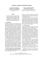
Figure 2: Accuracy curve on English development set
for lexicalized models.
coarse level conditions on {t
h
, d, σ}. For P

B
we
use three levels, which from fine to coarse are
{t
a
, w
h
, d, σ}, {t
a
, t
h
, d, σ} and {t
a
}. We follow
Collins (1999) to estimate P
A
and P
B
from a tree-
bank using a back-off strategy.
We use a simple approach to combine lexical
models with the unlexical hidden-state models we
obtained in the previous experiment. Namely, we
use a log-linear model that computes scores for
head-modifier sequences as
s(h, d, x
1:T
) = log P
sp
(x

1:T
|h, d) (21)
+ log P
det
(x
1:T
|h, d) ,
where P
sp
and P
det
are respectively spectral and
deterministic probabilistic models. We tested
combinations of each deterministic model with
the spectral unlexicalized model using different
number of states. Figure 2 shows the accuracies of
single deterministic models, together with combi-
nations using different number of states. In all
cases, the combinations largely improve over the
purely deterministic lexical counterparts, suggest-
ing that the information encoded in hidden states
is complementary to lexical preferences.
5.3 Results Analysis
We conclude the experiments by analyzing the
state space learned by the spectral algorithm.
Consider the space R
n
where the forward-state
vectors lie. Generating a modifier sequence corre-
sponds to a path through the n-dimensional state

space. We clustered sets of forward-state vectors
in order to create a DFA that we can use to visu-
alize the phenomena captured by the state space.
416
cc
jj dt nnp
prp$ vbg jjs
rb vbn pos
jj in dt cd
1
5
7
I
2
0
3
cc
nns
cd
,
$ nnp
cd nns
STOP
,
prp$ rb pos
jj dt nnp
9
$ nn
jjr nnp
STOP

STOP
cc
nn
STOP
cc
nn
,
prp$ nn pos
Figure 3: DFA approximation for the generation of NN
left modifier sequences.
To build a DFA, we computed the forward vec-
tors corresponding to frequent prefixes of modi-
fier sequences of the development set. Then, we
clustered these vectors using a Group Average
Agglomerative algorithm using the cosine simi-
larity measure (Manning et al., 2008). This simi-
larity measure is appropriate because it compares
the angle between vectors, and is not affected by
their magnitude (the magnitude of forward vec-
tors decreases with the number of modifiers gen-
erated). Each cluster i defines a state in the DFA,
and we say that a sequence x
1:t
is in state i if its
corresponding forward vector at time t is in clus-
ter i. Then, transitions in the DFA are defined us-
ing a procedure that looks at how sequences tra-
verse the states. If a sequence x
1:t
is at state i at

time t − 1, and goes to state j at time t, then we
define a transition from state i to state j with la-
bel x
t
. This procedure may require merging states
to give a consistent DFA, because different se-
quences may define different transitions for the
same states and modifiers. After doing a merge,
new merges may be required, so the procedure
must be repeated until a DFA is obtained.
For this analysis, we took the spectral model
with 9 states, and built DFA from the non-
deterministic automata corresponding to heads
and directions where we saw largest improve-
ments in accuracy with respect to the baselines.
A DFA for the automaton (NN, LEFT) is shown
in Figure 3. The vectors were originally divided
in ten clusters, but the DFA construction required
two state mergings, leading to a eight state au-
tomaton. The state named I is the initial state.
Clearly, we can see that there are special states
for punctuation (state 9) and coordination (states
1 and 5). States 0 and 2 are harder to interpret.
To understand them better, we computed an esti-
mation of the probabilities of the transitions, by
counting the number of times each of them is
used. We found that our estimation of generating
STOP from state 0 is 0.67, and from state 2 it is
0.15. Interestingly, state 2 can transition to state 0
generating prp$, POS or DT, that are usual end-

ings of modifier sequences for nouns (recall that
modifiers are generated head-outwards, so for a
left automaton the final modifier is the left-most
modifier in the sentence).
6 Conclusion
Our main contribution is a basic tool for inducing
sequential hidden structure in dependency gram-
mars. Most of the recent work in dependency
parsing has explored explicit feature engineering.
In part, this may be attributed to the high cost of
using tools such as EM to induce representations.
Our experiments have shown that adding hidden-
structure improves parsing accuracy, and that our
spectral algorithm is highly scalable.
Our methods may be used to enrich the rep-
resentational power of more sophisticated depen-
dency models. For example, future work should
consider enhancing lexicalized dependency gram-
mars with hidden states that summarize lexical
dependencies. Another line for future research
should extend the learning algorithm to be able
to capture vertical hidden relations in the depen-
dency tree, in addition to sequential relations.
Acknowledgements We are grateful to Gabriele
Musillo and the anonymous reviewers for providing us
with helpful comments. This work was supported by
a Google Research Award and by the European Com-
mission (PASCAL2 NoE FP7-216886, XLike STREP
FP7-288342). Borja Balle was supported by an FPU
fellowship (AP2008-02064) of the Spanish Ministry

of Education. The Spanish Ministry of Science and
Innovation supported Ariadna Quattoni (JCI-2009-
04240) and Xavier Carreras (RYC-2008-02223 and
“KNOW2” TIN2009-14715-C04-04).
417
References
Raphael Bailly. 2011. Quadratic weighted automata:
Spectral algorithm and likelihood maximization.
JMLR Workshop and Conference Proceedings –
ACML.
James K. Baker. 1979. Trainable grammars for speech
recognition. In D. H. Klatt and J. J. Wolf, editors,
Speech Communication Papers for the 97th Meeting
of the Acoustical Society of America, pages 547–
550.
Borja Balle, Ariadna Quattoni, and Xavier Carreras.
2012. Local loss optimization in operator models:
A new insight into spectral learning. Technical Re-
port LSI-12-5-R, Departament de Llenguatges i Sis-
temes Inform
`
atics (LSI), Universitat Polit
`
ecnica de
Catalunya (UPC).
Xavier Carreras. 2007. Experiments with a higher-
order projective dependency parser. In Proceed-
ings of the CoNLL Shared Task Session of EMNLP-
CoNLL 2007, pages 957–961, Prague, Czech Re-
public, June. Association for Computational Lin-

guistics.
Stephen Clark and James R. Curran. 2004. Parsing
the wsj using ccg and log-linear models. In Pro-
ceedings of the 42nd Meeting of the Association for
Computational Linguistics (ACL’04), Main Volume,
pages 103–110, Barcelona, Spain, July.
Michael Collins. 1999. Head-Driven Statistical Mod-
els for Natural Language Parsing. Ph.D. thesis,
University of Pennsylvania.
Arthur P. Dempster, Nan M. Laird, and Donald B. Ru-
bin. 1977. Maximum likelihood from incomplete
data via the em algorithm. Journal of the royal sta-
tistical society, Series B, 39(1):1–38.
Jason Eisner and Giorgio Satta. 1999. Efficient pars-
ing for bilexical context-free grammars and head-
automaton grammars. In Proceedings of the 37th
Annual Meeting of the Association for Computa-
tional Linguistics (ACL), pages 457–464, Univer-
sity of Maryland, June.
Jason Eisner and Noah A. Smith. 2010. Favor
short dependencies: Parsing with soft and hard con-
straints on dependency length. In Harry Bunt, Paola
Merlo, and Joakim Nivre, editors, Trends in Parsing
Technology: Dependency Parsing, Domain Adapta-
tion, and Deep Parsing, chapter 8, pages 121–150.
Springer.
Jason Eisner. 2000. Bilexical grammars and their
cubic-time parsing algorithms. In Harry Bunt and
Anton Nijholt, editors, Advances in Probabilis-
tic and Other Parsing Technologies, pages 29–62.

Kluwer Academic Publishers, October.
Joshua Goodman. 1996. Parsing algorithms and met-
rics. In Proceedings of the 34th Annual Meeting
of the Association for Computational Linguistics,
pages 177–183, Santa Cruz, California, USA, June.
Association for Computational Linguistics.
Daniel Hsu, Sham M. Kakade, and Tong Zhang. 2009.
A spectral algorithm for learning hidden markov
models. In COLT 2009 - The 22nd Conference on
Learning Theory.
Gabriel Infante-Lopez and Maarten de Rijke. 2004.
Alternative approaches for generating bodies of
grammar rules. In Proceedings of the 42nd Meet-
ing of the Association for Computational Lin-
guistics (ACL’04), Main Volume, pages 454–461,
Barcelona, Spain, July.
Terry Koo and Michael Collins. 2010. Efficient third-
order dependency parsers. In Proceedings of the
48th Annual Meeting of the Association for Compu-
tational Linguistics, pages 1–11, Uppsala, Sweden,
July. Association for Computational Linguistics.
Christopher D. Manning, Prabhakar Raghavan, and
Hinrich Sch
¨
utze. 2008. Introduction to Information
Retrieval. Cambridge University Press, Cambridge,
first edition, July.
Mitchell P. Marcus, Beatrice Santorini, and Mary A.
Marcinkiewicz. 1994. Building a large annotated
corpus of english: The penn treebank. Computa-

tional Linguistics, 19.
Andre Martins, Noah Smith, and Eric Xing. 2009.
Concise integer linear programming formulations
for dependency parsing. In Proceedings of the Joint
Conference of the 47th Annual Meeting of the ACL
and the 4th International Joint Conference on Natu-
ral Language Processing of the AFNLP, pages 342–
350, Suntec, Singapore, August. Association for
Computational Linguistics.
Takuya Matsuzaki, Yusuke Miyao, and Jun’ichi Tsujii.
2005. Probabilistic CFG with latent annotations. In
Proceedings of the 43rd Annual Meeting of the As-
sociation for Computational Linguistics (ACL’05),
pages 75–82, Ann Arbor, Michigan, June. Associa-
tion for Computational Linguistics.
Ryan McDonald and Fernando Pereira. 2006. Online
learning of approximate dependency parsing algo-
rithms. In Proceedings of the 11th Conference of
the European Chapter of the Association for Com-
putational Linguistics, pages 81–88.
Ryan McDonald, Fernando Pereira, Kiril Ribarov, and
Jan Hajic. 2005. Non-projective dependency pars-
ing using spanning tree algorithms. In Proceed-
ings of Human Language Technology Conference
and Conference on Empirical Methods in Natural
Language Processing, pages 523–530, Vancouver,
British Columbia, Canada, October. Association for
Computational Linguistics.
Gabriele Antonio Musillo and Paola Merlo. 2008. Un-
lexicalised hidden variable models of split depen-

dency grammars. In Proceedings of ACL-08: HLT,
Short Papers, pages 213–216, Columbus, Ohio,
June. Association for Computational Linguistics.
James D. Park and Adnan Darwiche. 2004. Com-
plexity results and approximation strategies for map
418
explanations. Journal of Artificial Intelligence Re-
search, 21:101–133.
Mark Paskin. 2001. Cubic-time parsing and learning
algorithms for grammatical bigram models. Techni-
cal Report UCB/CSD-01-1148, University of Cali-
fornia, Berkeley.
Slav Petrov and Dan Klein. 2007. Improved infer-
ence for unlexicalized parsing. In Human Language
Technologies 2007: The Conference of the North
American Chapter of the Association for Computa-
tional Linguistics; Proceedings of the Main Confer-
ence, pages 404–411, Rochester, New York, April.
Association for Computational Linguistics.
Slav Petrov, Leon Barrett, Romain Thibaux, and Dan
Klein. 2006. Learning accurate, compact, and in-
terpretable tree annotation. In Proceedings of the
21st International Conference on Computational
Linguistics and 44th Annual Meeting of the Asso-
ciation for Computational Linguistics, pages 433–
440, Sydney, Australia, July. Association for Com-
putational Linguistics.
Ivan Titov and James Henderson. 2006. Loss mini-
mization in parse reranking. In Proceedings of the
2006 Conference on Empirical Methods in Natu-

ral Language Processing, pages 560–567, Sydney,
Australia, July. Association for Computational Lin-
guistics.
Ivan Titov and James Henderson. 2007. A latent vari-
able model for generative dependency parsing. In
Proceedings of the Tenth International Conference
on Parsing Technologies, pages 144–155, Prague,
Czech Republic, June. Association for Computa-
tional Linguistics.
419