Excel 2019 pivot tables introduction to dashboards the step by step guide
Bạn đang xem bản rút gọn của tài liệu. Xem và tải ngay bản đầy đủ của tài liệu tại đây (26.88 MB, 173 trang )
2019 Microsoft Excel®
Pivot Tables &
Introduction To Dashboards
The Step-By-Step Guide
C.J. Benton
Copyright © 2019 C.J. Benton
All rights reserved.
No part of this publication may be reproduced, stored in a retrieval system, or
transmitted in any form or by any means, electronic, mechanical,
photocopying, recording, scanning, or otherwise without signed permission
from the author, except for the use of brief quotations for review purposes.
Limit Of Liability / Disclaimer Of Warranty: While the author has used their
best efforts in preparing this book, they make no representations or
warranties with respect to the accuracy or completeness of the contents of this
book. The author does not guarantee the reader’s results will match those of
the author. The advice and strategies contained herein may not be suitable
for your situation. The author is not engaged in offering financial, tax, legal
or other professional services by publishing this book. You should consult a
licensed professional where appropriate. The author shall not be liable for
any errors or omissions, loss of profit or any other commercial damages
including but not limited to special, incidental, consequential, or other
damages.
Trademarks: Microsoft and Excel are either registered trademarks or
trademarks of Microsoft Corporation in the United States and/or other
countries.
Thank you!
Thank you for purchasing and reading this book! Your feedback is valued
and appreciated. Please take a few minutes and leave a review.
More books by this author:
For a complete list please visit us at:
/>Excel® 2019 VLOOKUP The Step-By-Step Guide
Excel® 2016 The 30 Most Common Formulas & Features - The
Step-By-Step Guide
Excel® 2016 The VLOOKUP Formula in 30 Minutes The StepBy-Step Guide
The Step-By-Step Guide To The VLOOKUP formula in
Microsoft Excel® (version 2013)
Excel® Macros & VBA For Business Users - A Beginners Guide
Questions, comments?
Please contact us at:
Email:
Website: />
TABLE OF CONTENTS
CHAPTER 1
How To Use This Book
Files For Exercises
CHAPTER 2
Introduction To PivotTables
What Are PivotTables?
What Are The Main Parts Of A PivotTable?
CHAPTER 3
Creating your first PivotTable
Preparing the worksheet
The Recommended PivotTables feature
CHAPTER 4
Basic PivotTable Functionality
Summarizing Data
Why Do The ‘∑ Values’ Fields sometimes default to Count instead of Sum?
How To Drill-Down PivotTable Data
Adding Additional Rows (categories) To Your PivotTable
CHAPTER 5
Displaying Percentages In PivotTables
CHAPTER 6
Grouping PivotTable Data
Grouping Records
Count Function
CHAPTER 7
Slicers, Timelines, & Filtering
Timeline
Slicer
Report Connections
Formatting Timelines & Slicers
Ungrouping Date Data
Conditional Filters
Value Filters (Top & Bottom Performers)
Removing Filters
CHAPTER 8
Pivot Charts
Pie Chart Example
Quick Layout Options
Bar Chart Example
Value Filters & PivotCharts
Chart Styles
Stacked Bar Chart
Line Chart Example
Grouping Pivot Chart Date Data
Column Chart Example
Positive & Negative Values When Charting
CHAPTER 9
Ranking & Sorting PivotTable Results
CHAPTER 10
PivotTables from Imported Files & The Excel ® Data Model
The Excel ® Data Model
CHAPTER 11
Consolidating Data From Separate Workbooks To Create A Single PivotTable
Power Query
Append vs. Merge in Power Query
CHAPTER 12
Introduction To Dashboards
What is a Dashboard?
Dashboard Design
Dashboard Graphics
Doughnut Chart
>Doughnut Chart Example
Geographic (Maps)
>Map Example
Icons (Graphics)
>Icon Example
People (Add-Ins)
>People Graph Example
Sparklines
Icon Sets (Conditional Formatting)
CHAPTER 13
Social Media Dashboard Example
Preparing The Data
Adding Sparklines To The Dashboard
Conditional Formatting & Icon Sets
Formatting The Dashboard
CHAPTER 14
Auto Parts Dashboard Example
Adding Multiple PivotTables To A Single Workbook
Calculated Fields
Removing Or Changing Calculated Fields
Calculated Field Limitations
Adding Sparklines To The Dashboard
Adding a Chart To The Dashboard
Adding a Timeline To The Dashboard
Report Connections
CHAPTER 15
Refreshing PivotTable and Dashboard Data
Appending An Existing (internal) Data Source
Refresh vs. Refresh All
Overriding Existing Data (Manually)
Refreshing Data From An External Source
CHAPTER 16
Protecting Your Dashboard
Concealing Your PivotTable Source Data
Protecting The Dashboard Or Any Other Worksheet
Thank you!
More Books Available From This Author
Questions / Feedback
CHAPTER 1
HOW TO USE THIS BOOK
This book can be used as a tutorial or quick reference guide. It is intended
for users who are comfortable with the fundamentals of Microsoft Excel® and
are now ready to build upon this skill by learning PivotTables and
Dashboards.
This book assumes you already know how to create, open, save, and
modify an Excel® workbook and have a general familiarity with the Excel®
toolbar (Ribbon).
All of the examples in this book use Microsoft Excel® 2019, however
most of the functionality can be applied using Microsoft Excel® version
2016. All screenshots in this book use Microsoft Excel® 2019.
While this book provides several PivotTable examples, the book does
not cover ALL available Microsoft Excel® PivotTable features, formulas, and
functionality.
Please always back-up your work and save often. A good best
practice when attempting any new functionality is to create a copy of the
original spreadsheet and implement your changes on the copied
spreadsheet. Should anything go wrong, you then have the original
spreadsheet to refer back to. Please see the diagram below.
Diagram 1:
FILES FOR EXERCISES
The exercise files are available for download at the following website:
/>
CHAPTER 2
INTRODUCTION TO PIVOTTABLES
WHAT ARE PIVOTTABLES?
PivotTables are a feature within Microsoft Excel® that takes individual cells
or pieces of data and lets you arrange them into numerous types of calculated
views. These snapshots of summarized data, require minimal effort to create
and can be changed by simply clicking or dragging fields within your report.
By using built-in functions and filters, PivotTables allow you to
quickly organize and summarize large amounts of data. You can filter and
drill-down for more detailed examination of your numbers and various types
of analysis can be completed without the need to manually enter formulas
into the spreadsheet you’re analyzing.
For example, the below PivotTable is based on a detailed spreadsheet
of 3,888 individual records containing information about airplane parts. In
less than 1 minute, I was able to produce the following report for the quantity
of parts sold by region:
These PivotTable reports can also be formatted to improve readability.
However, formatting does require a little more time to complete.
Formatted example:
In today’s world with the massive amounts of information available,
you may be tasked with analyzing significant portions of this data. Perhaps
consisting of several thousand, hundreds of thousands, or even millions of
records. You may have to reconcile numbers from many different sources
and formats, such as assimilating material from:
Reports generated by another application, such as a legacy
system
Data imported into Excel® via a query from a database or other
application
Data copied or cut, and pasted into Excel® from the web or other
types of screen scraping activities
Analyzing test or research results from multiple subjects
Integrating information due to company mergers or acquisitions
One of the easiest ways to perform various and complex types of analysis and
reporting is to use PivotTables.
WHAT ARE THE MAIN PARTS OF A PIVOTTABLE?
Before we begin our first exercise, let’s review the three main components of
a PivotTable:
1. Rows: The rows section typically represents how you would like
to categorize or group your data. Some examples include:
employee name, region, department, part number etc.
2. Columns: The columns show the level or levels in which you’re
displaying your calculations. Often a time period such as a month,
quarter, or year, but can also be categories, product lines, etc.
3. Values: Values are the calculation portion of the report, these
figures can be sums, percentages, counts, averages, rankings or
custom computations.
CHAPTER 3
CREATING YOUR FIRST PIVOTTABLE
For our first exercise we’ll be using a month’s worth of police crime data.
Below is a sample, however due to space limitations the entire data set is
not displayed.
PREPARING THE WORKSHEET
When creating PivotTables, the best practice for each worksheet to be
analyzed is:
Contain no blank rows or columns inside your dataset
Have no merged cells
Each column heading has a unique name
For example:
To create a basic PivotTable, we’ll utilize Microsoft Excel’s®
‘Recommended PivotTables’ feature. This tool is useful when you need to
perform quick, high-level analysis, or are being asked for something ad hoc.
Typically, these reports are not formatted or distributed to a customer. To
illustrate how this functionality works, we’ll take the following spreadsheet
containing police crime data and summarize:
The total number of crimes by geographic location
For this exercise, we’ll take the PoliceCrimeData.xlsx spreadsheet containing
3,636 individual crime records and counting the number of unique ID fields
by Area. The Rows (our grouping) will be the geographic ‘AREA’ and the
Values (our calculation) will be a ‘COUNT’ of the ID records. In this
demonstration we will not have a Column level of detail.
WEB ADDRESS & FILE NAME FOR EXERCISE:
/>PoliceCrimeData.xlsx
THE RECOMMENDED PIVOTTABLES FEATURE
Below are the steps to create a basic PivotTable using Microsoft Excel’s®
Recommended PivotTables Feature, to begin:
1. Open the PoliceCrimeData.xlsx spreadsheet
2. Select columns A:D
3. From the Ribbon select Insert : Recommended PivotTables
The following dialogue box will appear:
4. Select the preview for ‘Count of ID by AREA’
5. Click the ‘OK’ button
A new report will be created counting the number of ID fields by area. Note:
this created a new worksheet, ‘Sheet1’ and the ‘PivotTable Fields’ pane on
the left side of the new worksheet.
Congratulations! You created your first PivotTable! In just a few short
minutes, you were able to quickly summarize the total number of crimes that
occurred for a time period by geographic area.
CHAPTER 4
BASIC PIVOTTABLE FUNCTIONALITY
Let’s build upon the fundamentals of creating and modifying a PivotTable,
by including multiple totals, viewing the details of a specific value, and
formatting our results for easier viewing.
EXAMPLE:
In this exercise we will take a spreadsheet containing fruit sale information
and:
Determine the total fruit sales by region and quarter
Display the individual fruit sales by region and quarter
WEB ADDRESS & FILE NAME FOR EXERCISE:
/>FruitSales.xlsx
SUMMARIZING DATA
Sample data for chapter 4, due to space limitations the entire data set is not
displayed.
First, we will determine the ‘total sales by region’ and then build upon this
by adding the ‘quarterly sales by region’:
1. Open the FruitSales.xlsx spreadsheet and select cells ‘A1:I65’
2. From the Ribbon select Insert : PivotTable
The following dialogue box will appear, please note the Data Range and
location where the new PivotTable will be located:
3. Click the ‘OK’ button
A new tab will be created and appear similar to the following. Note: the
‘PivotTable Fields’ pane on the left side of the new worksheet.
Next, we’ll categorize our report and select a calculation value.
4. In the ‘PivotTable Fields’ pane select the following fields:
REGION (Rows section)
TOTAL ( ∑ Values section)
WHY DO THE ‘∑ VALUES’ FIELDS SOMETIMES DEFAULT TO COUNT INSTEAD
OF SUM?
When PivotTable source data contains blank rows, for example when
selecting the entire column such as (Sheet1!$A:$ I ) instead of a specific cell
rage (Sheet1!$A$1:$ I $65), Excel® will default the calculation of a field
added to the ‘∑ Values’ section to count instead of sum.
If this happens, to change the ‘∑ Values’ section from count to sum:
Click the ‘Count of TOTAL’ drop-down arrow, then from the
sub-menu select ‘Value Field Settings…’
The following ‘Value Field Settings…’ dialogue box will appear:
From the ‘Summarize value field by’ list, select the ‘Sum’
option
Click the ‘OK’ button
Continuing with our example:
The following should be displayed on the right side of your screen. Note: the
format is not very easy to read.
5. We can change the column labels and format of the numbers. In
the below example:
Select cell ‘A3’ and change the text from ‘Row Labels’ to
‘REGION’
Select cell ‘B3’ and change the text from ‘Sum of TOTAL’
to ‘TOTAL SALES’
You may also change the currency format in cells ‘B4:B7’.
In the below example, the format was changed to U.S.
dollars with zero decimal places
Below is the formatted example:
To enhance the report further we’re going to going add Quarter columns.
This “level” dimension will provide greater detail of the total fruit sales.
6. Inside the ‘PivotTable Fields’ pane
field to the ‘Columns’ section.
drag
the ‘QUARTER’
IMPORTANT!
®
Excel is reading the ‘Quarter’ as a numeric value, therefore if you click,
instead of drag the field to the ‘Columns’ section, Excel® will apply a
calculation.
If this happens, click the drop-down arrow for ‘Sum of QUARTER’
in the ‘ ∑ Values’ section and select the option ‘Move to Column Labels’
We now have ‘QUARTER’ added to the summary
7. Select cell ‘B3’ and change the text from ‘Column Labels’ to
‘BY QUARTER’
8. The labels for cells ‘B4’, ‘C4’, ‘D4’, & ‘E4’ were changed by
adding the abbreviation text ‘QTR’ in front of each quarter
number
Before formatting:
After formatting:
HOW TO DRILL-DOWN PIVOTTABLE DATA
Before continuing with our example, let’s say you wanted to investigate
further why the Central Region’s Q1 results are so much higher than the East
& West regions.
PivotTables allow you to double-click on any calculated value to see the
detail of that cell. By double clicking the value, this will create a new
worksheet containing an Excel® table with the details of that cell.
For example, double-click on the calculated value in cell ‘B5’
To delete the table, right-click on ‘Sheet3’ and select ‘Delete’
You’ll receive the following message, click the ‘Delete’ button
ADDING ADDITIONAL ROWS (CATEGORIES) TO YOUR PIVOTTABLE
Lastly, we’ll review how to display the individual fruit sales by region and
quarter.
1. Drag the ‘QUARTER’ field from the ‘COLUMNS’ section to
the ‘ROWS’ section.