THE NORMALIZED CES PRODUCTION FUNCTION THEORY AND EMPIRICS pdf
Bạn đang xem bản rút gọn của tài liệu. Xem và tải ngay bản đầy đủ của tài liệu tại đây (1.29 MB, 52 trang )
WORKING PAPER SERIES
NO 1294 / FEBRUARY 2011
by Rainer Klump, Peter McAdam
and Alpo Willman
THE NORMALIZED
CES PRODUCTION
FUNCTION
THEORY AND
EMPIRICS
WORKING PAPER SERIES
NO 1294 / FEBRUARY 2011
THE NORMALIZED CES
PRODUCTION FUNCTION
THEORY AND EMPIRICS
1
by Rainer Klump
2
, Peter McAdam
3
and Alpo Willman
4
1 We thank Cristiano Cantore, Jakub Growiec, Olivier de La Grandville, Miguel León-Ledesma
and Ryuzo Sato for comments, past collaborations and support.
2 Goethe University, Frankfurt am Main & Center for Financial Studies.
3 European Central Bank, Kaiserstrasse 29, D-60311 Frankfurt am
Main, Germany: email: McAdam
is also visiting professor at the University of Surrey.
4 European Central Bank, Kaiserstrasse 29, D-60311
Frankfurt am Main, Germany: email:
Alpo.Willman@ecb. europa.eu
This paper can be downloaded without charge from or from the Social Science
Research Network electronic library at
NOTE: This Working Paper should not be reported as representing
the views of the European Central Bank (ECB).
The views expressed are those of the authors
and do not necessarily reflect those of the ECB.
In 2011 all ECB
publications
feature a motif
taken from
the €100 banknote.
© European Central Bank, 2011
Address
Kaiserstrasse 29
60311 Frankfurt am Main, Germany
Postal address
Postfach 16 03 19
60066 Frankfurt am Main, Germany
Telephone
+49 69 1344 0
Internet
Fax
+49 69 1344 6000
All rights reserved.
Any reproduction, publication and
reprint in the form of a different
publication, whether printed or produced
electronically, in whole or in part, is
permitted only with the explicit written
authorisation of the ECB or the authors.
Information on all of the papers published
in the ECB Working Paper Series can be
found on the ECB’s website, http://www.
ecb.europa.eu/pub/scientific/wps/date/
html/index.en.html
ISSN 1725-2806 (online)
3
ECB
Working Paper Series No 1294
February 2011
Abstract
4
Non technical summary
5
1 Introduction
7
2 The general normalized CES production
function and variants
11
2.1 Derivation via the power function
13
2.2 Derivation via the homogenous
production function
15
2.3 A graphical representation
15
2.4 Normalization as a means to uncover
valid CES representations
16
2.5 The normalized CES function
with technical progress
20
3 The elasticity of substitution as an engine
of growth
24
4 Estimated normalized production function
27
4.1 Estimation forms
34
4.2 The point of normalization – literally!
36
5 Normalization in growth and business
cycle models
38
6 Conclusions and future directions
40
References
43
CONTENTS
4
ECB
Working Paper Series No 1294
February 2011
Abstract. The elasticity of substitution between capital and labor and, in turn, the direction
of technical change are critical parameters in many fields of economics. Until recently, though,
the application of production functions with non-unitary substitution elasticities (i.e., non Cobb
Douglas) was hampered by empirical and theoretical uncertainties. As has recently been re-
vealed, “normalization” of production functions and production-technology systems holds out
the promise of resolving many of those uncertainties. We survey and critically assess the in-
trinsic links between production (as conceptualized in a macroeconomic production function),
factor substitution (as made most explicit in Constant Elasticity of Substitution functions) and
normalization (defined by the fixing of baseline values for relevant variables). First, we recall
how the normalized CES function came into existence and what normalization implies for its
formal properties. Then we deal with the key role of normalization in recent advances in the
theory of business cycles and of economic growth. Next, we discuss the benefits normalization
brings for empirical estimation and empirical growth research. Finally, we identify promising
areas of future research on normalization and factor substitution.
Keywords. Normalization, Constant Elasticity of Substitution Production Function, Factor-
Augmenting Technical Change, Growth Theory, Identification, Estimation.
5
ECB
Working Paper Series No 1294
February 2011
Non-technical Summary
Substituting scarce factors of production by relatively more abundant ones is a key
element of economic efficiency and a driving force of economic growth. A measure
of that force is the elasticity of substitution between capital and labor which is the
central parameter in production functions, and in particular CES (Constant Elas-
ticity of Substitution) ones. Until recently, the application of production functions
with non-unitary substitution elasticities (i.e., non Cobb Douglas) was hampered
by empirical and theoretical uncertainties.
As has recently been revealed, “normalization” of production functions and
production-technology systems holds out the promise of resolving many of those
uncertainties and allowing elements as the role of the substitution elasticity and
biased technical change to play a deeper role in growth and business-cycle anal-
ysis. Normalization essentially implies representing the production function in
consistent indexed number form. Without normalization, it can be shown that
the production function parameters have no economic interpretation since they
are dependent on the normalization point and the elasticity of substitution itself.
This feature significantly undermines estimation and comparative-static exer-
cises, among other things. Due to the central role of the substitution elasticity in
many areas of dynamic macroeconomics, the concept of CES production functions
has recently experienced a major revival. The link between economic growth and
the size of the substitution elasticity has long been known. As already demon-
strated by Solow (1956) in the neoclassical growth model, assuming an aggregate
CES production function with an elasticity of substitution above unity is the easiest
way to generate perpetual growth. Since scarce labor can be completely substi-
tuted by capital, the marginal product of capital remains bounded away from zero
in the long run.
Nonetheless, the case for an above-unity elasticity appears empirically weak and
theoretically anomalous. However, when analytically investigating the significance
of non-unitary factor substitution and non-neutral technical change in dynamic
macroeconomic models, one faces the issue of “normalization”, even though the
issue is still not widely known. The (re)discovery of the CES production function in
normalized form in fact paved the way for the new and fruitful, theoretical and em-
pirical research on the aggregate elasticity of substitution which has been witnessed
over the last years. In La Grandville (1989b) and Klump and de La Grandville
(2000) the concept of normalization was introduced in order to prove that the
aggregate elasticity of substitution between labor and capital can be regarded as
6
ECB
Working Paper Series No 1294
February 2011
an important and meaningful determinant of growth in the neoclassical growth
model.
In the meantime this approach has been successfully applied in a series of
theoretical papers to a wide variety of topics. Further, as Klump et al. (2007a,
2008) demonstrated, normalization also has been a breakthrough for empirical
research on the parameters of aggregate CES production functions, in particular
when coupled with the system estimation approach. Empirical research has long
been hampered by the difficulties in identifying at the same time an aggregate
elasticity of substitution as well as growth rates of factor augmenting technical
change from the data. The received wisdom, in both theoretical and empirical
literatures, suggests that their joint identification is infeasible. Accordingly, for
more than a quarter of a century following Berndt (1976), common opinion held
that the US economy was characterized by aggregate Cobb-Douglas technology,
leading, in turn, to its default incorporation in economic models (and, accordingly,
the neglect of possible biases in technical progress). Translating normalization into
empirical production-technology estimations allows the presetting of the capital
income share (or, if estimated, facilitates the setting of reasonable initial parameter
conditions); it provides a clear correspondence between theoretical and empirical
production parameters and allows us ex post validation of estimated parameters.
Here we analyze and survey the intrinsic links between production (as concep-
tualized in a macroeconomic production function), factor substitution (as made
most explicit in CES production functions) and normalization.
7
ECB
Working Paper Series No 1294
February 2011
Until the laws of thermodynamics are repealed, I shall continue to relate
outputs to inputs - i.e. to believe in production functions.
Samuelson (1972) (p. 174)
All these results, negative and depressing as they are, should not sur-
prise us. Bias in technical progress is notoriously difficult to identify.
Kennedy and Thirwall (1973) (p. 784)
The degree of factor substitution can thus be regarded as a determinant
of the steady state just as important as the savings rate or the growth
rate of the labor force.
Klump et al. (2008) (p. 655)
1 Introduction
Substituting scarce factors of production by relatively more abundant ones is a key
element of economic efficiency and a driving force of economic growth. A measure
of that force is the elasticity of substitution between capital and labor which is the
central parameter in production functions, and in particular CES (Constant Elas-
ticity of Substitution) ones. Until recently, the application of production functions
with non-unitary substitution elasticities (i.e., non Cobb Douglas) was hampered
by empirical and theoretical uncertainties. As has recently been revealed, “nor-
malization” of production functions and production-technology systems holds out
the promise of resolving many of those uncertainties and allowing considerations as
the role of the substitution elasticity and biased technical change to play a deeper
role in growth and business-cycle analysis. Normalization essentially implies rep-
resenting the production function in consistent indexed number form. Without
normalization, it can be shown that the production function parameters have no
economic interpretation since they are dependent on the normalization point and
the elasticity of substitution itself. This feature significantly undermines estima-
tion and comparative-static exercises, among other things.
Let us first though place the importance of the topic in perspective. Due to
the central role of the substitution elasticity in many areas of dynamic macroe-
conomics, the concept of CES production functions has recently experienced a
major revival. The link between economic growth and the size of the substitution
elasticity has long been known. As already demonstrated by Solow (1956) in the
neoclassical growth model, assuming an aggregate CES production function with
8
ECB
Working Paper Series No 1294
February 2011
an elasticity of substitution above unity is the easiest way to generate perpetual
growth. Since scarce labor can be completely substituted by capital, the marginal
product of capital remains bounded away from zero in the long run. Nonetheless,
the case for an above-unity elasticity appears empirically weak and theoretically
anomalous.
1
It has been shown that integration into world markets is also a feasible way
for a country to increase the effective substitution between factors of production
and thus pave the way for sustained growth (Ventura (1997), Klump (2001), Saam
(2008)). On the other hand, it can be shown in several variants of the standard neo-
classical (exogenous) growth model that introducing an aggregate CES production
functions that with an elasticity of substitution below unity can generate multiple
growth equilibria, development traps and indeterminacy (Azariadis (1996), Klump
(2002), Kaas and von Thadden (2003)), Guo and Lansing (2009)).
Public finance and labor economics are other fields where the elasticity of sub-
stitution has been rediscovered as a crucial parameter for understanding the impact
of policy changes. This relates to the importance of factor substitution possibili-
ties for the demand for each input factor. As pointed out by Chirinko (2002), the
lower the elasticity of substitution, the smaller the response of business investment
to variations in interest rates caused by monetary or fiscal policy.
2
In addition,
the welfare effects of tax policy changes specifically, appear highly sensitive to
the assumed values of the substitution elasticity. Rowthorn (1999) also stresses
its importance in macroeconomic analysis of the labor market and, in particu-
lar, how incentives for higher investment formation exercise a significant effect on
unemployment when the elasticity of substitution departs from unity.
Indeed, there is now mounting empirical evidence that aggregate production is
better characterized by a non-unitary elasticity of substitution (rather than unitary
or above unitary), e.g., Chirinko et al. (1999), Klump et al. (2007a), Le´on-Ledesma
et al. (2010a). Chirinko (2008)’s recent survey suggests that most evidence favors
elasticities ranges of 0.4-0.6 for the US. Moreover, Jones (2003, 2005)
3
argued that
capital shares exhibit such protracted swings and trends in many countries as to
1
The critical threshold level for the substitution elasticity (to generate such perpetual growth)
can be shown to be increasing in the growth of labor force and decreasing in the saving rate, see
La Grandville (1989b).
2
This may be one reason why estimated investment equations struggle to identify interest-rate
channels.
3
Jones’ work essentially builds on Houthakker (1955)’s idea that production combinations
reflect the (Pareto) distribution of innovation activities, Jones proposes a “nested” production
function. Given such parametric innovation activities, this will exhibit a (far) less than unitary
substitution elasticity over business-cycle frequencies but asymptote to Cobb-Douglas.
9
ECB
Working Paper Series No 1294
February 2011
be inconsistent with Cobb-Douglas or CES with Harrod-neutral technical progress
(see also Blanchard (1997), McAdam and Willman (2011a)).
This coexistence of capital and labor-augmenting technical change, has differ-
ent implications for the possibility of balanced or unbalanced growth. A balanced
growth path - the dominant assumption in the theoretical growth literature - sug-
gests that variables such as output, consumption, etc tend to a common growth
rate, whilst key underlying ratios (e.g., factor income shares, capital-output ra-
tio) are constant, Kaldor (1961). Neoclassical growth theory suggests that, for
an economy to posses a steady state with positive growth and constant factor in-
come shares, the elasticity of substitution must be unitary (i.e., Cobb Douglas) or
technical change be Harrod neutral.
As Acemoglu (2009) (Ch. 15) comments, however, there is little reason to
assume technical change is necessarily labor augmenting.
4
In models of “biased”
technical change (e.g., Kennedy (1964), Samuelson (1965), Acemoglu (2003), Sato
(2006)), scarcity, reflected by relative factor prices, generates incentives to invest
in factor-saving innovations. In other words, firms reduce the need for scarce
factors and increase the use of abundant ones. Acemoglu (2003) further suggested
that while technical progress is necessarily labor-augmenting along the balanced
growth path, it may become capital-biased in transition. Interestingly, given a
below-unitary substitution elasticity this pattern promotes the stability of income
shares while allowing them to fluctuate in the medium run.
However, when analytically investigating the significance of non-unitary factor
substitution and non-neutral technical change in dynamic macroeconomic models,
one faces the issue of “normalization”, even though the issue is still not widely
known. The (re)discovery of the CES production function in normalized form in
fact paved the way for the new and fruitful, theoretical and empirical research
on the aggregate elasticity of substitution which has been witnessed over the last
years.
In La Grandville (1989b) and Klump and de La Grandville (2000) the concept
of normalization was introduced in order to prove that the aggregate elasticity
of substitution between labor and capital can be regarded as an important and
meaningful determinant of growth in the neoclassical growth model. In the mean-
time this approach has been successfully applied in a series of theoretical papers
(Klump (2001), Papageorgiou and Saam (2008), Klump and Irmen (2009), Xue
4
Moreover, that a BGP cannot coexist with capital augmentation is becoming increasingly
questioned in the literature, see Growiec (2008), La Grandville (2010), Leon-Ledesma and Satchi
(2010).
10
ECB
Working Paper Series No 1294
February 2011
and Yip (2009), Guo and Lansing (2009), Wong and Yip (2010)) to a wide variety
of topics.
A particular striking example of how neglecting normalization can significantly
bias results and how explicit normalization can help to overcome those biases is
presented in Klump and Saam (2008). The effect of a higher elasticity of substi-
tution on the speed of convergence in a standard Ramsey type growth model is
shown to double if a non-normalized (or implicitly normalized) CES function is
replaced by a reasonably normalized one.
Further, as Klump et al. (2007a, 2008) demonstrated, normalization also has
been a breakthrough for empirical research on the parameters of aggregate CES
production functions,
5
in particular when coupled with the system estimation ap-
proach. Empirical research has long been hampered by the difficulties in identifying
at the same time an aggregate elasticity of substitution as well as growth rates
of factor augmenting technical change from the data. The received wisdom, in
both theoretical and empirical literatures, suggests that their joint identification
is infeasible. Accordingly, for more than a quarter of a century following Berndt
(1976), common opinion held that the US economy was characterized by aggregate
Cobb-Douglas technology, leading, in turn, to its default incorporation in economic
models (and, accordingly, the neglect of possible biases in technical progress).
6
Translating normalization into empirical production-technology estimations al-
lows the presetting of the capital income share (or, if estimated, facilitates the
setting of reasonable initial parameter conditions); it provides a clear correspon-
dence between theoretical and empirical production parameters and allows us ex
post validation of estimated parameters. In a series of papers, Le´on-Ledesma
et al. (2010a,b) showed the empirical advantages in estimating and identifying
production-technology systems when normalized. Further, McAdam and Willman
(2011b) showed that normalized factor-augmenting CES estimation, in the context
of estimating “New Keynesian” Phillips curves, helped better identify the volatil-
ity in the driving variable (real marginal costs) that most previous researchers had
not detected.
Here we analyze the intrinsic links between production (as conceptualized in a
5
It should be noted that the advantages of re-scaling input data to ease the computational
burden of highly nonlinear regressions has been the subject of some study, e.g., ten Cate (1992).
And some of this work was in fact framed in terms of production-function analysis, De Jong
(1967), De Jong and Kumar (1972). See also Cantore and Levine (2011) for a novel discussion
of alternative but equivalent ways to normalize.
6
It should be borne in mind, however, that Berndt’s result concerned only the US manufac-
turing sector.
11
ECB
Working Paper Series No 1294
February 2011
macroeconomic production function), factor substitution (as made most explicit in
CES production functions) and normalization. The paper is organized as follows.
In section 2 we recall how the CES function came into existence and what this
implies for its formal properties. Sections 3 and 4 will deal with the role of normal-
ization in recent advances in the theory of business cycles and economic growth.
Section 5 will discuss the merits normalization brings for empirical growth research.
The last section concludes and identifies promising area of future research.
2 The general normalized CES production
function and variants
It is common knowledge that the first rigid derivation of the CES production
function appeared in the famous Arrow et al. (1961) paper (hereafter ACMS ).
7
However, there were important forerunners, in particular the explicit mentioning
of a CES type production technology (with an elasticity of substitution equal to
2) in the Solow (1956) article (done, Solow wrote, to add a “bit of variety”) on
the neoclassical growth model. There was also the hint to a possible CES func-
tion in its Swan (1956) counterpart (on the Swan story see Dimond and Spencer
(2008)).
8
Shortly before, though, Dickinson (1954) (p. 169, fn 1) had already
made use of a CES production technology in order to model “a more general kind
of national-income function, in which the factor shares are variable” compared to
the Cobb-Douglas form. It has even been conjectured that the famous and mys-
terious tombstone formula of von Th¨unen dealing with “just wages” can be given
a meaningful economic interpretation if it is regarded as derived from an implicit
CES production function with an elasticity of substitution equal to 2 (see Jensen
(2010)).
In this section we want to demonstrate, that (and how) the formal construction
of a CES production function is intrinsically linked to normalization. The function
7
It is still not widely known that the famous Arrow et al. (1961) paper was in fact the merging
of two separate submissions to the Review of Economics and Statistics following a paper from
Arrow and Solow, and another from Chenery and Minhas.
8
In the inaugural ANU Trevor Swan Distinguished Lecture, Peter L. Swan (Swan (2006))
writes, “While Trevor was at MIT he pointed out that a production function Solow was utilizing
had the constant elasticity of substitution, CES, property In this way, the CES function was
officially born. Solow and his coauthors publicly thanked Trevor for this insight (see Arrow et
al, 1961).”
12
ECB
Working Paper Series No 1294
February 2011
may be defined as follows:
Y
t
= F (K
t
,N
t
)=C
πK
σ−1
σ
t
+(1− π) N
σ−1
σ
t
σ
σ−1
(1)
where distribution parameter π ∈ (0, 1) reflects capital intensity in production; C
is an efficiency parameter and, σ, is the elasticity of substitution between capital,
K, and labor, N. Like all standard CES functions, equation (1) nests a Cobb-
Douglas function when σ → 1; a Leontief function with fixed factor proportions
when σ = 0; and a linear production function with perfect factor substitution
when σ = ∞.
The construction of such an aggregate production technology with a CES prop-
erty starts from the formal definition of the elasticity of substitution which had
been introduced independently by Hicks (1932) and Robinson (1933) (on the dif-
ferences between both approaches to the concept see Hicks (1970)). It is there
defined (in the case of two factors of production, capital and labor) as the elastic-
ity of K/N with respect to the marginal rate of substitution between K and N
(the percentage change in factor proportions due to a change in the marginal rate
of technical substitution) along an isoquant:
9
σ ∈ [0, ∞]=
d (K/N) / (K/N)
d (F
N
/F
K
) / (F
N
/F
K
)
=
d log (K/N)
d log (F
N
/F
K
)
(2)
As Hicks notes this concept of elasticity can be equally expressed in terms of
the second derivative of the production function, but only under the assumption
of constant returns to scale (due to Euler’s theorem).
Since under this assumption the marginal factor productivities would also equal
factor prices and the marginal rate of substitution would be identical with the
wage/capital rental ratio, the elasticity of substitution can also expressed as the
elasticity of income per person y with respect to the marginal product of labor in
efficiency terms (or the real wage rate, w), i.e., Allen’s theorem (Allen (1938)).
Given that income per person is a linear homogeneous function y = f (k)ofthe
capital intensity k = K/N, the elasticity of substitution can also be defined as:
σ =
dy
dw
·
w
y
= −
f
(κ)[f (κ) − κf
(κ)]
κf (κ) f
(κ)
(3)
9
Alternatively, the substitution elasticity is sometimes expressed in terms of the parameter
of factor substitution, ρ ∈ [−1, ∞], where ρ =
1−σ
σ
.
13
ECB
Working Paper Series No 1294
February 2011
Although it is rarely stated explicitly, the elasticity of substitution is implicitly
always defined as a point elasticity. This means that it is related to one particular
baseline point on one particular isoquant (see our Figures 1 and 2 below). From
there a whole system of non-intersecting isoquants is defined which all together
create the CES production function. Even if it is true that a given and constant
elasticity of substitution would not change along a given isoquant or within a given
system of isoquants, it is also evident that changes in the elasticity of substitution
would of course alter the system of isoquants. Following such a change in the
elasticity of substitution the old and the new isoquant are not intersecting at the
baseline point but are tangents, if the production function is normalized. And they
should not intersect because given the definition of the elasticity of substitution
(i.e. the percentage change in factor proportions due to a change in the marginal
rate of technical substitution) at this particular point (as in all other points which
are characterized by the same factor proportion) the old and the new CES function
should still be characterized by the same factor proportion and the same marginal
rate of technical substitution.
Just as there are two possible definitions of σ following (3) - from
dy
dw
·
w
y
and from
−
f´(k)[f(k)−kf´(k)]
kf´´´(k)f(k)
- thus there are two ways of uncovering the normalized production
function. These, we cover in the following two sub-sections.
2.1 Derivation via the Power Function
Let us start from the definition σ =
d log (y)
d log (w)
=
dy
dw
·
w
y
, integration of which gives the
power function,
y = cw
σ
(4)
where c is some integration constant.
10
Under the assumption of constant returns
to scale (or perfectly competitive factor and product markets), and applying the
profit-maximizing condition that the real wage equals the marginal product of
labor, and with the application of Allen’s theorem, we can transform this equation
into the form y = c
y − k
dy
dk
σ
.
Accordingly, after integration and simplification, this leads us to a production
10
ACMS started from the empirical observation that the relationship between per-capital in-
come and the wage rate might best be described with the help of such a power function. Note,
σ = 1 implies a linear relationship between y and w which would, in turn, imply that labor’s
share of income was constant. However, instead of a linear y − w scatter plot, they found a con-
cave relationship in the US data. The authors then tested a logarithmic and power relationship
and concluded that σ<1. Integration of power function (4) then leads to a production function
with constant elasticity of substitution, consistent with definitions (2), (3).
14
ECB
Working Paper Series No 1294
February 2011
function with the constant elasticity of substitution function (see La Grandville
(2009), p. 83ff for further details):
y =
βk
σ−1
σ
+ α
σ
σ−1
(5)
and,
Y =
βK
σ−1
σ
+ αL
σ−1
σ
σ
σ−1
(6)
in the extensive form.
It should be noted that (5) and (6) contain the two constants of integration
β and α = c
−
1
σ
, where the latter directly depends on σ. Identification of these
two constants make use of baseline values for the power function (4) and for the
functional form (5) at the given baseline point in the system of isoquant. In a
dynamic setting this baseline point must (as we will see later) also be regarded as
a particular point in time, t = t
0
:
y
0
= cw
σ
0
(7)
y
0
=
βk
σ−1
σ
+ α
σ
σ−1
(8)
Together with (5) this leads to the normalized CES production function,
y = y
0
π
0
k
k
0
σ−1
σ
+(1− π
0
)
σ
σ−1
(9)
and,
Y = Y
0
π
0
K
K
0
σ−1
σ
+(1− π
0
)
N
N
0
σ−1
σ
σ
σ−1
(10)
in the extensive form. Parameter π
0
=
y
0
−w
0
y
0
=
r
0
K
0
Y
0
denotes the capital share in
total income at the point of normalization.
11
As a test of consistent normalization,
we see from (10) that for t = t
0
we retrieve Y = Y
0
.
11
Under perfect competition, this distribution parameter is equal to the capital income share
but, under imperfect competition with non-zero aggregate mark-up, it equals the share of capital
income over total factor income.
15
ECB
Working Paper Series No 1294
February 2011
2.2 Derivation via the Homogenous Production Function
It was shown by Paroush (1964), Yasui (1965) and McElroy (1967) that the rather
narrow assumption of Allen’s theorem is not essential for the derivation of the CES
production function which can start directly from the original Hicks definition (2).
This definition can be transformed into a second-order differential equation whose
solution also implies two constants of integration.
Following Klump and Preissler (2000) we start with the definition of the elas-
ticity of substitution in the case of linear homogenous production function Y
t
=
F (K
t
,N
t
)=N
t
f (k
t
)wherek
t
= K
t
/N
t
is the capital-labor ratio in efficiency
units. Likewise y
t
= Y
t
/N
t
represents per-capita production.
The definition of the substitution elasticity, σ = −
f´(k)[f(k)−kf´(k)]
kf´´´(k)f(k)
, can then be
viewed as a second-order differential equation in k having the following general
CES production function as its solution (intensive and extensive forms):
y
t
= a
k
σ−1
σ
t
+ b
σ
σ−1
(11)
Y
t
= a
K
σ−1
σ
t
+ bN
σ−1
σ
t
σ
σ−1
(12)
where parameters a and b are two arbitrary constants of integration with the
following correspondence with the parameters in equation (1): C = a (1 + b)
σ
σ−1
and π =1/ (1 + b).
A meaningful identification of these two constants is given by the fact that the
substitution elasticity is a point elasticity relying on three baseline values: a given
capital intensity k
0
= K
0
/N
0
, a given marginal rate of substitution [F
K
/F
N
]
0
=
w
0
/r
0
and a given level of per-capita production y
0
= Y
0
/N
0
. Accordingly, (1)
becomes,
Y
t
= Y
0
π
0
K
t
K
0
σ−1
σ
+(1− π
0
)
N
t
N
0
σ−1
σ
σ
σ−1
(13)
where π
0
= r
0
K
0
/ (r
0
K
0
+ w
0
N
0
) is the capital income share evaluated at the point
of normalization. Rutherford (2003) calls (13) (or (10)) the “calibrated form”.
2.3 A Graphical Representation
Normalization as understood by La Grandville (1989b), Klump and de La Grandville
(2000) and Klump and Preissler (2000) is again nothing else but identifying these
two arbitrary constants in an economically meaningful way. Normalizing means
16
ECB
Working Paper Series No 1294
February 2011
the fixing (in the K − N plane as in Figure 1) of a baseline point (which can
be thought of as a point in time at, t = t
0
), characterized by specific values of
N,K, Y and the marginal rate of technical substitution μ
0
- in which isoquants of
CES functions with different elasticities of substitution but with all other param-
eters equal - are tangents.
Normalization is helpful to clarify the conceptual relationship between the elas-
ticity of substitution and the curvature of the isoquants of a CES production func-
tion (see La Grandville (1989a) for a discussion of various misunderstandings on
this point). Klump and Irmen (2009) point out that in the point of normaliza-
tion (and only there), there exists an inverse relationship between the elasticity
of substitution and the curvature of isoquant of the normalized CES production
function. This relationship has also an interpretation in terms of the degree of
complementarity of both input factors. At the normalization point, a higher elas-
ticity of substitution implies a lower degree of complementarity between the input
factors. The link between complementarity between input factors and the elas-
ticity of substitution is also discussed in Acemoglu (2002) and in Nakamura and
Nakamura (2008).
Equivalently (in the k − y plane as in Figure 2) the baseline point can be
characterized by specific values of k, y and the marginal productivity of capital (or
the real wage rate). If base values for these three variables are selected this means
of course that also a baseline value for the elasticity of production with respect
to capital input is fixed which (under perfect competition) equals capital share in
total income.
2.4 Normalization As A Means To Uncover Valid CES
Representations
Normalization thus creates specific ‘families’ of CES functions whose members all
share the same baseline point but are distinguished by the elasticity of substitution
(and only the elasticity of substitution).
17
ECB
Working Paper Series No 1294
February 2011
Figure 1. Isoquants of Normalized CES Production Functions
Figure 2. Normalized per-capita CES production functions
y
1
0.5
V
1
1
V
1
V
of
0
V
1
V
V
of
0
Y
0
N
0
K
0
P
K
N
18
ECB
Working Paper Series No 1294
February 2011
As shown in Klump and Preissler (2000), normalization also helps to distinguish
those variants of CES production functions which are functionally identical with
the general form (1) from those which are inconsistent with (5) in one way or
another. Consider, first, the “standard form” of the CES production function, as
it was introduced by ACMS, restated below:
Y = C
πK
σ−1
σ
+(1− π) N
σ−1
σ
σ
σ−1
(14)
This variant is clearly identical with (10), albeit (and this is a crucial aspect)
with the “substitution parameter” C and the “distribution parameter” π being
defined in the following way (solving for completeness in terms of both ρ and σ):
C (σ, ·)=Y
0
[π
0
K
ρ
0
+(1− π
0
) N
ρ
0
]
ρ
= Y
0
r
0
K
1/σ
0
+ w
0
N
1/σ
0
r
0
K
0
+ w
0
N
0
σ
σ−1
(15)
π (σ, ·)=
π
0
K
ρ
0
π
0
K
ρ
0
+(1− π
0
) N
ρ
0
=
r
0
K
1/σ
0
r
0
K
1/σ
0
+ w
0
N
1/σ
0
(16)
Expressions (15) and (16) reveal that, in the non-normalized case, both “parame-
ters” (apart from being dependent on the scale of the normalized variables) change
with variations in the elasticity of substitution, unless K
0
and N
0
are exactly equal,
implying k
0
=1.
This makes the non-normalized form in general inappropriate for comparative
static exercises in the substitution elasticity. It is the interaction between the nor-
malized efficiency and distribution terms and the elasticity of substitution which
guarantees that within one family of CES functions the members are only dis-
tinguished by the elasticity of substitution. Given the accounting identity (and
abstracting from the presence of an aggregate mark-up),
Y
0
= r
0
K
0
+ w
0
N
0
(17)
it also follows from this analysis that treating C and π in (14) as deep parameters is
equivalent to assuming k
0
= 1. In the case σ → 0, we have a perfectly symmetrical
Leontief function.
As explained in Klump and Saam (2008) the Leontief case can serve as a
benchmark for the choice of the normalization values for k
0
in calibrated growth
models. The baseline capital intensity corresponds to the capital intensity that
would be efficient if the economy’s elasticity of substitution were zero. For k<
19
ECB
Working Paper Series No 1294
February 2011
k
0
the economy’s relative bottleneck resides in this case in its capacity to make
productive use of additional labor, as capital is the relatively scarce factor. For
k>k
0
the same is true for capital and labor is relatively scarce. Since the latter
case is most characteristic for growth model of capitalist economies, calibrations
of these model can be based on the assumption k>k
0
.
In the following sub-sections, we will illustrate how normalization can reveal
whether certain production functions used in the literature are legitimate.
2.4.1 David and van de Klundert (1965) Version
Consider the CES variant proposed by David and van de Klundert (1965):
Y =
(BK)
σ−1
σ
+(AN)
σ−1
σ
σ
σ−1
(18)
This variant is identical with (10) as long as the two “efficiency levels” are defined
in the following way:
B =
Y
0
K
0
π
σ
σ−1
0
(19)
A =
Y
0
N
0
(1 − π
0
)
σ
σ−1
(20)
Again, it is obvious, that the efficiency levels change directly with the elasticity of
substitution.
2.4.2 Ventura (1997) Version
Consider now a CES variant used by Ventura (1997):
Y =
K
σ−1
σ
+(AN)
σ−1
σ
σ
σ−1
(21)
At first glance (21) could be regarded as a special case of (14) with B being equal
to one. With a view on the normalized efficiency level it becomes clear, however,
that B = 1 is not possible for given baseline values and a changing elasticity of
substitution. Given that Ventura (1997) makes use of (21) in order to study the
impact of changes in the elasticity of substitution on the speed of convergence,
in the light of this inconsistency his results should be regarded with particular
caution. As shown in Klump (2001), Ventura’s result are unnecessarily restrictive;
working with a correctly normalized CES technology leads to much more general
results.
20
ECB
Working Paper Series No 1294
February 2011
2.4.3 Barro and Sala-i-Martin (2004) Version
Next consider the CES production function proposed by Barro and Sala-i-Martin
(2004):
Y = C
π (BK)
σ−1
σ
+(1− π) ((1 − B) N)
σ−1
σ
σ
σ−1
(22)
Normalization is helpful in this case in order to show that (22) can be transformed
without any problems into (10) and/or (14) so that the terms B and 1 − B simply
disappear. If for any reason these two terms are considered necessary elements of
a standard CES production function, they cannot be chosen independently from
the normalized values for C and π, but they remain independent from changes in
σ.
2.5 The Normalized CES Function with Technical Progress
So far we have treated efficiency levels as constant over time. If we now consider
factor-augmenting technical progress one has to keep in mind the intrinsic links
between rising factor efficiency in the distribution of income. This brings us to
one further justification for normalizing CES production function which is closely
related to the concept of neutral technical progress and was first articulated by
Kamien and Schwartz (1968). Normalization implies that there may be considered
a reference (or representative) value for the capital income share (and thus for
income distribution) at some given point. Technical progress that does not changes
income distribution over time is called Harrod-Neutral technical progress. There
are many other types of classifiable neutral technical change, however, that would
not have this effect.
12
So the whole concept of whether technical progress is neutral
with respect to the income distribution, relies on the idea that one has to check
whether or not a given income distribution at one point in time remains constant.
This given income distribution, which is used to evaluate possible distribution
effect of technical progress, is exactly the income distribution in the baseline point
of normalization at a fixed point in time, t = t
0
.
12
See the seminal contribution of Sato and Beckmann (1970) for such a classification.
21
ECB
Working Paper Series No 1294
February 2011
2.5.1 Constant growth rates of normalized factor efficiency levels
As shown in Klump et al. (2007a), a normalized CES production function with
factor-augmenting technical progress can be written as,
Y =
E
K
t
K
σ−1
σ
+
E
N
t
N
σ−1
σ
σ
σ−1
(23)
where E
K
t
and E
N
t
represent the levels of efficiency of both input factors.
13
Thus, whereas the ACMS specification seems to imply that technological change
is always Hicks-neutral, the above specification allows for different growth rates
of factor efficiency. To circumvent problems related to Diamond-McFadden’s Im-
possibility theorem (Diamond et al. (1978); Diamond and McFadden (1965)), we
assume a certain functional form for the growth rates of both efficiency levels and
define:
E
i
t
= E
i
0
e
γ
i
(t−t
0
)
(24)
where γ
i
denotes growth in technical progress associated with factor i and t repre-
sents a (typically linear) time trend. The combination γ
K
= γ
N
> 0 denotes Hicks-
Neutral technical progress; γ
K
> 0,γ
N
= 0 yields Solow-Neutrality; γ
K
=0,γ
N
> 0
represents Harrod-Neutrality; and γ
K
> 0 = γ
N
> 0 indicates general factor-
augmenting technical progress.
14
E
i
0
are the fixed points of the two efficiency levels, taken at the common baseline
time, t = t
0
. Again, normalization of the CES function implies that members of
the same CES family should all share the same fixed point and should in this
point and at that time of reference only be characterized by different elasticities
of substitution. In order to ensure that this property also holds in the presence of
13
In the case where there is such technical progress, the question of whether σ is greater than or
below unity takes on added importance. Recall, when σ<1, factors are “gross complements” in
production and “gross substitutes” otherwise. Thus, it can be shown that with gross substitutes,
substitutability between factors allows both the augmentation and bias of technological change
to favor the same factor. For gross complements, however, a capital-augmenting technological
change, for instance, increases demand for labor (the complementary input) more than it does
capital, and vice versa. By contrast, when σ = 1 an increase in technology does not produce
a bias towards either factor (factor shares will always be constant since any change in factor
proportions will be offset by a change in factor prices).
14
Neutrality concepts associate innovations to related movements in marginal products and
factor ratios. An innovation is Harrod-Neutral if relative input shares remain unchanged for a
given capital-output ratio. This is also called labor-augmenting since technical progress raises
production equivalent to an increase in the labor supply. More generally, for F (X
i
,X
j
, , A),
technical progress is X
i
-augmenting if F
A
A = F
X
i
X
i
.
22
ECB
Working Paper Series No 1294
February 2011
growing factor efficiencies, it follows that:
E
N
0
=
Y
0
N
0
1
1 − π
0
σ
1−σ
; E
K
0
=
Y
0
K
0
1
π
0
σ
1−σ
(25)
Note that at t = t
0
,e
γ
i
(t−t
0
)
= 1. This ensures that at the common fixed point the
factor shares are not biased by the growth of factor efficiencies but are just equal
to the distribution parameters π
0
and 1 − π
0
Inserting equations (24) and the normalized values (25) into (23), leads to a
normalized CES function that can be rewritten in the following form that again
resembles the ACMS variant:
Y =
π
0
Y
0
K
0
· e
γ
K
(t−t
0
)
· K
t
σ−1
σ
+(1− π
0
)
Y
0
N
0
· e
γ
N
(t−t
0
)
· N
t
σ−1
σ
σ
σ−1
(26)
or equivalently,
Y = Y
0
π
0
K
1−σ
σ
0
K
t
· e
γ
K
(t−t
0
)
σ−1
σ
+(1− π
0
) N
1−σ
σ
0
N
t
· e
γ
N
(t−t
0
)
σ−1
σ
σ
σ−1
(27)
In this specification of the normalized CES function, with factor augmenting tech-
nical progress, the growth of efficiency levels for capital and labor is now measured
by the expressions K
0
e
γ
K
(t−t
0
)
and N
0
e
γ
N
(t−t
0
)
, respectively, and t
0
is the baseline
year. Again, we see from (27) that for t = t
0
we retrieve Y = Y
0
.
Special cases of (27) are the specifications used by Rowthorn (1999), Bentolila
and Saint-Paul (2003) or Acemoglu (2002), where N
0
= K
0
= Y
0
= 1 is implicitly
assumed, or by Antr`as (2004) who sets N
0
= K
0
= 1. Caballero and Hammour
(1998), Blanchard (1997) and Berthold et al. (2002) work with a version of (27)
where in addition to N
0
= K
0
=1,γ
K
= 0 is also assumed so that technological
change is only of the labor-augmenting variety.
It is also worth noting that for constant efficiency levels γ
N
= γ
K
=0our
normalized function (27) is formally identical with the CES function that Jones
(2003) (p. 12) has proposed for the characterization of the “short term”. In his
terminology, the normalization values k
0
, y
0
,andπ
0
are “appropriate” values of
the fundamental production technology that determines long-run dynamics. This
long-run production function is then considered to be of a Cobb-Douglas form with
constant factor shares equal to π
0
and 1−π
0
and with a constant exogenous growth
rate. Actual behavior of output and factor input is thus modeled as permanent
23
ECB
Working Paper Series No 1294
February 2011
fluctuations around “appropriate” long-term values. For a similar approach in
which steady state Cobb-Douglas parameter values are used to normalized a CES
production function see Guo and Lansing (2009).
2.5.2 Growth Rates in Normalized Technical Progress Functions:
Time-Varying Frameworks
Following recent theoretical discussion about possible biases in technical progress
(e.g., Acemoglu (2002)), it is not clear that growth rates of technical progress com-
ponents should always be constant. An innovation of Klump et al. (2007a) was to
allow deterministic but time-varying technological progress terms where curvature
or decay terms could be uncovered from the data in economically meaningful ways.
For this they used a Box and Cox (1964) transformation in a normalized context
where (with E
i
t
= e
g
i
):
g
i
(γ
i
,λ
i
,t,t
0
)=
γ
i
λ
i
t
0
t
t
0
λ
i
− 1
,i= K, N (28)
Curvature parameter λ
i
determines the shape of the technical progress function.
For λ
i
= 1, technical progress functions, g
i
, are the (textbook) linear specification;
if 0 <λ
i
< 1 they are exponential; if λ
i
= 0 they are log-linear and λ
i
< 0they
are hyperbolic functions in time. Note, the re-scaling of γ
i
and t by the fixed point
value t
0
in (28) allows us to interpret γ
N
and γ
K
directly as the rates of labor- and
capital-augmenting technical change at the fixed-point period.
Asymptotically, function (28) would behave as follows:
g
i
(γ
i
,λ
i
,t,t
0
)=
lim
t→∞
g
i
= ∞ for λ
i
≥ 0
lim
t→∞
g
i
= −
γ
i
λ
i
t
0
for λ
i
< 0
∂g
i
∂t
= γ
i
t
t
0
λ
i
−1
⇒
∂g
i
∂t
= γ
i
for λ
i
=1
∂g
i
∂t
=0 for λ
i
< 1
This framework allows the data to decide on the presence and dynamics of factor-
augmenting technical change rather than being imposed a priori by the researcher.
If, for example, the data supported an asymptotic steady state, this would arise
from the estimated dynamics of these curvature functions (i.e., labor-augmenting
technical progress becomes dominant (linear), that of capital absent or decaying).
24
ECB
Working Paper Series No 1294
February 2011
In addition, as McAdam and Willman (2011a) pointed out, the framework
also allows one to nest various strands of economic convergence paths towards the
steady state. For instance, the combination,
γ
N
> 0,λ
N
=1; γ
K
=0,λ
K
=0 (29)
coupled with the assumption, σ>>1, corresponds to that drawn upon by Ca-
ballero and Hammour (1998) and Blanchard (1997), in explaining the decline in
the labor income share in continental Europe.
Another combination speculatively termed “Acemoglu-Augmented” Technical
Progress by McAdam and Willman (2011a), can be nested as,
γ
N
,γ
K
> 0; λ
N
=1,λ
K
< 1 (30)
where σ<1 is more natural.
Consider two cases within (30). A “weak” variant, λ
K
< 0, implies that the
contribution of capital augmentation to TFP is bounded with its growth com-
ponent returning rapidly to zero; a “strong” case, where 0 <λ
K
< 1, capital
imparts a highly persistent contribution with (asymptotic convergence to) a zero
growth rate. Both cases are asymptotically consistent with a balanced growth
path (BGP), where TFP growth converges to that of labor-augmenting technical
progress, γ
N
. The interplay between |γ
N
− γ
K
| and λ
K
,λ
N
and can thus be con-
sidered sufficient statistics of BGP divergence. Normalization, moreover, makes
this kind of classification quite natural since we are looking at biases in technical
progress relative to some average or representative point.
3 The elasticity of substitution as an engine of
growth
Although one of the first references to a CES structure of aggregate production
appears in the Solow (1956) paper it had been for a long time impossible to an-
swer the question of what effect changes in the substitution elasticity had on the
steady-state values in the standard neoclassical growth model. Common sense
would certainly suggest that easier factor substitution - via helping to overcome
decreasing returns - should lead to a higher level of development. But a formal
proof of this conjecture seemed out of reach. In fact, when Harbrecht (1975) tried
to answer this question with the help of a (non-normalized) David and van de