Identifying a time dependent zeroth order coefficient in a time fractional diffusion wave equation by using the measured data at a boundary point 2
Bạn đang xem bản rút gọn của tài liệu. Xem và tải ngay bản đầy đủ của tài liệu tại đây (2.81 MB, 27 trang )
Applicable Analysis
An International Journal
ISSN: (Print) (Online) Journal homepage: />
Identifying a time-dependent zeroth-order
coefficient in a time-fractional diffusion-wave
equation by using the measured data at a
boundary point
Ting Wei & Kaifang Liao
To cite this article: Ting Wei & Kaifang Liao (2021): Identifying a time-dependent zeroth-order
coefficient in a time-fractional diffusion-wave equation by using the measured data at a boundary
point, Applicable Analysis, DOI: 10.1080/00036811.2021.1932834
To link to this article: />
Published online: 27 May 2021.
Submit your article to this journal
Article views: 4
View related articles
View Crossmark data
Full Terms & Conditions of access and use can be found at
/>
APPLICABLE ANALYSIS
/>
Identifying a time-dependent zeroth-order coefficient in a
time-fractional diffusion-wave equation by using the measured
data at a boundary point
Ting Wei
and Kaifang Liao
School of Mathematics and Statistics, Lanzhou University, Lanzhou, People’s Republic of China
ABSTRACT
ARTICLE HISTORY
In this paper, we investigate a nonlinear inverse problem of identifying
a time-dependent zeroth-order coefficient in a time-fractional diffusionwave equation by using the measured data at a boundary point. We firstly
prove the existence, uniqueness and regularity of the solution for the corresponding direct problem by using the contraction mapping principle. Then
we try to give a conditional stability estimate for the inverse zeroth-order
coefficient problem and propose a simple condition for the initial value and
zeroth-order coefficient such that the uniqueness of the inverse coefficient
problem is obtained. The Levenberg–Marquardt regularization method is
applied to obtain a regularized solution. Based on the piecewise linear finite
elements approximation, we find an approximate minimizer at each iteration by solving a linear system of algebraic equations in which the Fréchet
derivative is obtained by solving a sensitive problem. Two numerical examples in one-dimensional case and two examples in two-dimensional case
are provided to show the effectiveness of the proposed method.
Received 5 June 2020
Accepted 12 May 2021
COMMUNICATED BY
D. XU
KEYWORDS
Time-fractional
diffusion-wave equation;
time-dependent
zeroth-order coefficient;
uniqueness; conditional
stability;
Levenberg–Marquardt
regularization method
2010 MATHEMATICS
SUBJECT
CLASSIFICATIONS
35R30; 65M32
1. Introduction
Let 1 < α < 2. Suppose ⊂ Rd , d = 1, 2, 3 be a bounded domain whose boundary ∂ is sufficiently
smooth. Let the unknown function u satisfy the following time-fractional diffusion-wave equation,
initial conditions and boundary conditions
⎧ α
∂ u(x, t) + Au(x, t) + p(t)q(x, t)u(x, t) = f (x, t), x ∈ , 0 < t ≤ T,
⎪
⎪
⎨ 0+
u(x, 0) = ϕ(x),
x∈ ,
(1)
u
(x,
0)
=
ψ(x),
x
∈ ,
⎪
t
⎪
⎩
∂ν u(x, t) = 0,
x ∈ ∂ , 0 < t ≤ T,
α is the Caputo fractional left-sided derivative given in Kilbas et al. [1] and Podlubny [2] as
where ∂0+
α
∂0+
u(x, t) =
CONTACT Ting Wei
1
(2 − α)
© 2021 Informa UK Limited, trading as Taylor & Francis Group
t
0
uss (x, s)(t − s)1−α ds,
t > 0,
2
T. WEI AND K. LIAO
in which (·) is the Gamma function, and the second-order elliptic operator A is defined by
d
Au(x, t) = −
∂xi aij (x)∂xj u(x, t) ,
i,j=1
in which the coefficients aij (x) = aji (x) ∈ C1 ( ¯ ), 1 ≤ i, j ≤ d satisfy
d
aij (x)ξi ξj ≥ c0 |ξ |2 ,
x∈ ¯,
ξ ∈ Rd ,
c0 > 0,
i,j=1
and
d
∂ν u(x, t) =
aij (x)∂xj u(x, t) νi (x),
x∈∂ ,
i,j=1
for the unit outward normal vector ν(x) = (ν1 (x), . . . , νd (x)) at x ∈ ∂ .
If all functions except u in problem (1) are given, it is a well-posed direct problem. This model can
be used to formulate the anomalous superdiffusion phenomena of particles in heterogenous porous
media, see [3–5] for some application backgrounds. However, sometimes the time-dependent zerothorder coefficient p(t) may not know, for example the diffusion of pollutants in underground sandy
soil, if the particles of pollutants are absorbed on the surface of sand stone such that the particles do
not have random walks or have a chemical reaction such that the pollutants are degraded, then the
zeroth-order term in mathematical equation is appeared where the coefficient p(t) is called absorbtion
coefficient or reaction coefficient which describes the absorbtion rate or reaction rate of pollutants, i.e
the amount of absorbed or degraded pollutants in unit volume at unit time. Generally, it is difficult to
know the exact coefficient p(t). We want to identify it based on an additional condition. In this paper,
we consider an inverse problem for identifying the zeroth-order coefficient p(t) in problem (1). The
additional condition is
u(x0 , t) = g(t),
x0 ∈ ∂ ,
0 ≤ t ≤ T.
(2)
Direct problems for time-fractional diffusion-wave equations have been investigated widely in
various aspects, for examples, the existence and uniqueness of weak solutions [6–8], numerical
methods [9–13].
For inverse problems of time-fractional diffusion-wave equations, there are not so many references. In [14], the authors consider a backward problem for a time-fractional diffusion-wave equation
and use the Tikhonov regularization method to solve it. Siskova and Slodicka in [15] investigate an
inverse time-dependent source problem by an additional integral condition. In [16], Liao et al. consider an inverse time-dependent source problem by an additional boundary condition. All the studies
mentioned before focused on the linear inverse problems for the time-fractional diffusion-wave
equations.
In this paper, we try to solve a nonlinear inverse problem of recovering the time-dependent coefficient p(t). We firstly give the existence, uniqueness and regularity result for the corresponding
direct problem by using a fixed point theorem and then prove a conditional stability estimate for
the inverse problem. A numerical algorithm is provided to give a regularized approximate solution.
For a similar problem on a time-fractional diffusion equation, Fujishiro et al. in [17] identified a
zeroth-order coefficient from the measured data at an interior or a boundary point, and obtained
a stability result, however, no numerical method is provided. Zhang in [18] determined a timedependent diffusion coefficient from the Neumann data at a boundary data in a time-fractional
diffusion equation and gave the uniqueness of inverse problem and an efficient algorithm. In [19], Sun
et al. considered to seek a time-dependent potential coefficient in a multi-term time-fractional diffusion equation and used the Levenberg–Marquardt regularization method to solve the corresponding
APPLICABLE ANALYSIS
3
inverse problem numerically. In [20], Sun et al. investigated a time-dependent convection coefficient
in a time-fractional diffusion equation.
There are four different points compared with the references. For the direct problem, the Fourier
method is fail to give an explicit expression of the solution for problem (1) since the zeroth-order
coefficient is concerned with variable t. Secondly, we obtain a higher regularity of solution for the
direct problem compared with ones in [17, 19] such that the Caputo derivative is well defined in a
pointwise meaning, in fact the solutions for the integral equations in [19] may not be the solutions
of the corresponding direct problems. On the other hand, we give a conditional stability estimate for
this inverse zeroth-order coefficient problem which is a new issue as we know. Finally, we propose a
numerical method combined with a finite element approximation to solve this inverse problem.
Throughout this paper, if unspecified, we always use the following assumptions
p(t) ∈ L∞ (0, T),
(3)
∞
q(x, t) ∈ L (0, T; D(A)),
(4)
and ψ(x) ∈ D(A1−1/α )
ϕ(x) ∈ D(A)
(5)
∞
f ∈ L (0, T; D(A)).
(6)
This paper is organized as follows. We present some preliminaries in Section 2. In Section 3, we give
the existence, uniqueness and regularity of the solution for the direct problem. In Section 4, we give a
stability estimate and a conditional stability estimate for the inverse problem. In Section 5, we use the
Levenberg–Marquardt regularization method combined with the linear finite element discretization
to find an approximate time-dependent zeroth-order coefficient. Numerical results for four examples
in one- and two-dimensional cases are provided to illustrate the efficiency of our used method in
Section 6. Finally, we give a brief conclusion in Section 7.
2. Preliminaries
In this paper, the space AC[0, T] is the space of absolutely continuous functions on [0, T]. And define
ACn [0, T] := {z(t)|z ∈ Cn−1 [0, T], z(n−1) (t) ∈ AC[0, T]},
n ≥ 2.
Denote the norms in L2 ( ) and L∞ (0, T) as · = · L2 ( ) , · ∞ = · L∞ (0,T) , and the inner
product in L2 ( ) as (·, ·). H s ( ), s ∈ R is the standard Sobolev space (see Adams [21]).
We define the operator A = A + 1 in D(A) := {u ∈ H 2 ( )|∂ν u = 0on∂ }, then by the standard
theorems on second-order elliptic equations we know A is a self-adjoint and positive operator. Let
{λk , φk }∞
k=1 be an eigensystem of A in D(A), then we have 0 < λ1 < λ2 ≤ λ3 ≤ · · · , limk→∞ λk =
2
∞, Aφk = λk φk , and suppose {φk }∞
k=1 ⊂ D(A) be an orthonormal basis of L ( ).
γ
We can define the Hilbert scale space D(A ) for γ ≥ 0 (see, e.g. [22]) by
∞
γ
2
2γ
λk |(ψ, φk )|2 < ∞ ,
D(A ) = ψ ∈ L ( );
k=1
Aγ ψ =
∞
γ
λk (ψ, φk )φk ,
ψ ∈ D(Aγ ),
k=1
equipped with the norm ψ
D(Aγ )
= Aγ ψ
D(Aγ ) ⊂ H 2γ ( ),
0 ≤ γ ≤ 1,
C1 ψ
D(Aγ )
H 2γ ( )
≤ ψ
≤ C2 ψ
L2 ( ) . According to
H 2γ ( ) ,
[23, 24], we have
ψ ∈ D(Aγ ),
0 ≤ γ ≤ 1,
1 3
γ = , .
4 4
4
T. WEI AND K. LIAO
Definition 2.1 ([1]): Let f (t) ∈ AC[0, T] for α ∈ (0, 1) and f (t) ∈ AC2 [0, T] for α ∈ (1, 2). The
α f is defined by
Caputo left-sided fractional derivative ∂0+
α
f (t) =
∂0+
t
1
(1 − α)
0
f (s)
ds,
(t − s)α
0 < t ≤ T,
0 < α < 1,
and
α
f (t) =
∂0+
1
(2 − α)
f (s)
ds,
(t − s)α−1
t
0
0 < t ≤ T,
1 < α < 2.
Lemma 2.1 ([25]): Let f ∈ Lp (0, T) and g ∈ Lq (0, T) with 1 ≤ p, q ≤ ∞ and 1/p + 1/q = 1. Then
t
the function f ∗ g defined by f ∗ g(t) = 0 f (t − s)g(s) ds belongs to C[0, T] and satisfies
|f ∗ g(t)| ≤ f
Lp (0,t)
g
Lq (0,t) ,
t ∈ [0, T].
Lemma 2.2 ([25]): Let u, v ∈ H 2 ( ) and d ≤ 3. Then uv ∈ H 2 ( ) with the estimate
uv
with C > 0 depending on u
H2 ( )
≤C v
(7)
H2 ( )
H2 ( ) .
Lemma 2.3 ([17]): Let C, α > 0 and u, d ∈ L1 (0, T) be nonnegative functions satisfying
u(t) ≤ Cd(t) + C
t
0
(t − s)α−1 u(s) ds,
t ∈ (0, T).
(t − s)α−1 d(s) ds,
t ∈ (0, T).
Then we have
u(t) ≤ Cd(t) + C
t
0
Lemma 2.4 ([26]): Let a, b, α > 0 be constants and u ∈ L1 (0, T) be nonnegative functions satisfying
u(t) ≤ a + b
t
0
(t − s)α−1 u(s) ds,
a.e. t ∈ (0, T).
Then we have
u(t) ≤ aEα,1 (b (α))1/α t α ≤ C0 a,
a.e. t ∈ (0, T),
where C0 > 0 is a constant depending on b, α, T.
Definition 2.2 ([1]): The Mittag-Leffler function is
∞
Eα,β (z) =
k=0
zk
,
(αk + β)
z ∈ C,
where α > 0 and β ∈ R are arbitrary constants.
Proposition 2.1 ([1]): Let 0 < α < 2 and β ∈ R be arbitrary. We suppose that μ is such that π α/2 <
μ < min{π , π α}. Then there exists a constant C = C(α, β, μ) > 0 such that
| Eα,β (z) |≤
C
,
1+ | z |
μ ≤| arg(z) |≤ π.
APPLICABLE ANALYSIS
5
Proposition 2.2 (See [8]): Let α > 0, λ > 0, then we have
d
(Eα,1 (−λt α )) = −λt α−1 Eα,α (−λt α ),
dt
t > 0.
Proposition 2.3 ([1]): Let 1 < α < 2, λ > 0, then we have
d
(tEα,2 (−λt α )) = Eα,1 (−λt α ), t > 0,
dt
d α−1
Eα,α (−λt α )) = t α−2 Eα,α−1 (−λt α ),
(t
dt
t > 0.
Lemma 2.5 ([8]): For λ > 0 and 1 < α < 2 then we have
α
∂0+
(tEα,2 (−λt α )) = −λtEα,2 (−λt α ),
t > 0,
and
α
(Eα,1 (−λt α )) = −λEα,1 (−λt α ),
∂0+
t > 0.
Lemma 2.6 ([16]): Let 1 < α < 2 and h(t) ∈ AC[0, T]. Define
t
p(t) :=
0
h(τ )(t − τ )α−1 Eα,α (−λ(t − τ )α ) dτ ,
t > 0.
If λ > 0, then p(t) ∈ AC2 [0, T] satisfies
α
∂0+
p(t) + λp(t) = h(t),
0 < t ≤ T,
(8)
and if λ = 0, then p(t) ∈ AC2 [0, T] satisfies
α
∂0+
t
0
h(τ )(t − τ )α−1 dτ = (α)h(t),
Lemma 2.7: Let 0 < α < 1. Suppose f ∈ W 1,∞ (0, T) and f
α
f
∂0+
C[0,T]
≤ C1 E1α f
0 < t ≤ T.
L∞ (0,T)
(9)
≤ E1 , then we have
1−α
C[0,T] ,
(10)
where C1 = C1 (α) > 0 is independent of f.
α f ∈ C[0, T] and
Proof: By Lemma 2.1, we know ∂0+
α
|∂0+
f (t)| ≤
=
1
f
(1 − α)
1
f
(2 − α)
t
L∞ (0,T)
L∞ (0,T) t
0
1
ds
(t − s)α
1−α
,
0 < t ≤ T,
(11)
α f (0) = 0.
that means ∂0+
If E1 = 0, we know f (t) = 0 for t ∈ [0, T] almost every, which deduces easily the result (10). In
the following, we suppose E1 > 0.
Denote t0 = f C[0,T] /E1 . We have to consider two cases.
(1) If t0 ≥ T, then by (11), we can obtain
α
f (t)| ≤
|∂0+
1
f
(2 − α)
L∞ (0,T) T
1−α
6
T. WEI AND K. LIAO
1
f L∞ (0,T) t01−α
(2 − α)
1
0 ≤ t ≤ T.
Eα f 1−α
C[0,T] ,
(2 − α) 1
≤
=
(2) If t0 < T, then by (11), we have
1
f L∞ (0,T) t01−α
(2 − α)
1
0 ≤ t ≤ t0 .
Eα f 1−α
C[0,T] ,
(2 − α) 1
α
|∂0+
f (t)| ≤
=
(12)
For t0 < t ≤ T, by using the integration by parts, we can obtain
α
f (t)| =
|∂0+
=
≤
1
(1 − α)
t−t0
0
f (s)
ds +
(t − s)α
t
t−t0
f (s)
ds
(t − s)α
t−t0
1
f (t − t0 )t0−α − f (0)t−α − α
(1 − α)
1
4 f
(1 − α)
−α
C[0,T] t0
1
f
1−α
+
0
f (s)
ds +
(t − s)α+1
1−α
L∞ (0,T) t0
,
t
t−t0
f (s)
ds
(t − s)α
t0 ≤ t ≤ T.
Putting the value of t0 into the inequality above and combining with (12), we get the estimate (10).
Lemma 2.8: Let 1 < α < 2. Suppose f ∈ W 2,∞ (0, T) and f
W 2,∞ (0,T)
2+α
α
∂0+
f
C[0,T]
≤ C2 E2 4
≤ E2 , then we have
2−α
4
f
C[0,T] ,
(13)
where C2 = C2 (α, T) > 0 is independent of f.
Proof: By Definition 2.1, for α ∈ (1, 2), we know
α−1
α
∂0+
f (t) = ∂0+
f (t).
(14)
From the condition f ∈ W 2,∞ (0, T) ⊂ C1 [0, T], we know f ∈ W 1,∞ (0, T) and
f W 2,∞ (0,T) ≤ E2 , by Lemma 2.7, we have
α
f
∂0+
C[0,T]
≤ C1 (α)E2α−1 f
f
2−α
C[0,T] .
L∞ (0,T)
≤
(15)
By the interpolation theorems in Adames [21] ( See Theorem 5.8 in page 140, Theorem 5.2 in page
135), we have two estimates for f (t) as
f
L∞ (0,T)
1
2
≤ K1 f
f
H 1 (0,T)
1
2
(16)
L2 (0,T)
and
f
L2 (0,T)
≤ f
H 1 (0,T)
≤ 2K2 f
1/2
H 2 (0,T)
f
1/2
,
L2 (0,T)
(17)
where K1 , K2 are constants independent of f. Substituting (17) into (16), we have
f
L∞ (0,T)
≤
√
√
2K1 K2 f
3
4
H 2 (0,T)
f
1
4
L2 (0,T)
≤
√
√
1 3
2K1 K2 T 2 E24 f
1
4
L∞ (0,T) ,
(18)
APPLICABLE ANALYSIS
in which we use f
1
L2 (0,T)
≤ T2 f
L∞ (0,T) . Putting (18)
into (15), we have
2+α
α
f
∂0+
C[0,T]
7
≤ C2 (α, T)E2 4
2−α
4
f
C[0,T] .
(19)
3. Existence, uniqueness and regularity of solution for the direct problem
In this section, by the fixed point theorem, we can obtain the following existence, uniqueness and
regularity results for problem (1). Throughout this paper, the notation C means a generic constant
independent of u which may take a different value appearing everywhere.
Theorem 3.1: Let conditions (3)–(6) hold. Then the integral Equation (23) has a unique solution u ∈
C([0, T]; D(A)) ∩ C1 ([0, T]; L2 ( )) satisfying
u
C([0,T];D(A))
≤ C( ϕ
+ u
D(A)
C1 ([0,T];L2 ( ))
+ ψ
D(A1−1/α )
+ Au
+ f
C([0,T];L2 ( ))
L∞ (0,T;D(A)) ),
(20)
where C > 0 is depending on α, T, p ∞ and q L∞ (0,T;D(A)) .
Moreover, if f ∈ AC([0, T]; L2 ( )), p ∈ AC[0, T], q ∈ AC([0, T]; D(A)), then there is a unique
α u∈
solution to the direct problem (1) satisfying u ∈ AC2 ([0, T]; L2 ( )) ∩ C([0, T]; D(A)) and ∂0+
2
C([0, T]; L ( )), and we have the following estimate
α
∂0+
u
C([0,T];L2 ( ))
with C > 0 depending on α, T, p
is depending only Ep .
≤ C( ϕ
∞
and q
D(A)
+ ψ
D(A1−1/α )
L∞ (0,T;D(A)) .
+ f
L∞ (0,T;D(A)) ),
Further, if p
∞
(21)
≤ Ep , then the constant C
Proof: Rewrite the first equation in problem (1) as
α
u(x, t) + Au(x, t) = f (x, t) + b(x, t)u(x, t),
∂0+
(22)
where b(x, t) = (1 − p(t)q(x, t)).
We define the operator-valued functions
∞
(ϕ, φk )Eα,1 (−λn t α )φk (x),
S1 (t)ϕ =
t > 0,
n=1
∞
(ψ, φk )tEα,2 (−λn t α )φk (x),
S2 (t)ψ =
t > 0,
n=1
∞
(h, φk )t α−1 Eα,α (−λn t α )φk (x),
S3 (t)h =
t > 0.
n=1
Based on the Fourier method, refer to [8], we know the solution for problem (1) satisfies the following
integral equation
u(x, t) = S1 (t)ϕ + S2 (t)ψ +
t
0
S3 (t − τ )f (·, τ ) dτ +
t
0
S3 (t − τ )(b(·, τ )u(·, τ )) dτ .
(23)
8
T. WEI AND K. LIAO
By Lemma 2.1, we know
∞
2
D(A)
S1 (t)ϕ
=
(ϕ, φn )2 λ2n Eα,1 (−λn t α )2 ≤ C ϕ
2
D(A) ,
(24)
n=1
where C > 0 is a constant depending on α.
Since the Mittag-Leffler function Eα,1 (−λn t α ) is continuous over t ≥ 0, then by the uniform
convergence theorem, we know S1 (t)ϕ ∈ C([0, T]; D(A)). By Lemma 2.2, we have
∞
(ϕ, φn )(−λn t α−1 )Eα,α (−λn t α )φn (x),
∂t (S1 (t)ϕ) =
(25)
n=1
then by Lemma 2.1 and maxs≥0 [sγ /(1 + s)] ≤ 1 for γ ∈ [0, 1], we have
∞
2
∂t (S1 (t)ϕ)
(ϕ, φn )2 (−λn t α−1 )2 Eα,α (−λn t α )2 ,
=
n=1
∞
≤C
(ϕ, φn )2 ((λn t α )1−1/α /(1 + λn t α ))2 λn ,
2/α
n=1
≤C ϕ
2
D(A1/α )
≤C ϕ
2
D(A) ,
(26)
where C is depending on α. Thus we know ∂t (S1 (t)ϕ) ∈ C([0, T]; L2 ( )) and further S1 (t)ϕ ∈
C1 ([0, T]; L2 ( )). The following estimate holds
S1 (t)ϕ
C1 ([0,T];L2 ( ))
+ S1 (t)ϕ
C([0,T];D(A))
≤ Cϕ
D(A) ,
(27)
where C is depending on α.
Similarly, we have
S2 (t)ψ
D(A)
≤C ψ
D(A1−1/α ) ,
(28)
and S2 (t)ϕ ∈ C([0, T]; D(A)). By Lemma 2.3, we have
∞
∂t (S2 (t)ϕ) =
(ψ, φn )Eα,1 (−λn t α )φn (x),
(29)
n=1
it deduces by Lemma 2.1 that
∂t (S2 (t)ψ) ≤ C ψ ,
(30)
and S2 (t)ψ ∈ C([0, T]; D(A)) ∩ C1 ([0, T]; L2 ( )) and
S2 (t)ψ
C([0,T];D(A))
+ S2 (t)ψ
C1 ([0,T];L2 ( ))
≤C ψ
D(A1−1/α ) ,
(31)
where C is depending on α.
t
t
α−1 E
α
Denote u3 (x, t) = 0 S3 (t − τ )f (·, τ ) dτ = ∞
α,α (−λn (t − τ ) )(f (·, τ ), φn )
n=1 0 (t − τ )
dτ φn (x), by Lemma 2.1 and the Cauchy inequality, it follows that
∞
u3 (·, t)
2
D(A)
=
n=1
t
0
(t − τ )α−1 Eα,α (−λn (t − τ )α )(f (·, τ ), φn ) dτ
2
λ2n ,
APPLICABLE ANALYSIS
∞
≤ CT 2α−1
T
n=1 0
(f (·, τ ), φn )2 λ2n dτ ≤ C f
2
L2 (0,T;D(A))
< ∞,
9
(32)
thus by Lemma 2.1 and the uniform convergence theorem, we know u3 ∈ C([0, T]; D(A)).
By Lemma 2.3, we have
∞
∂t u3 (x, t) =
t
n=1 0
(t − τ )α−2 Eα,α−1 (−λn (t − τ )α )(f (·, τ ), φn ) dτ φn (x),
(33)
then we have
∞
2
∂t u3 (·, t)
t
=
0
n=1
(t − τ )α−2 Eα,α−1 (−λn (t − τ )α (f (·, τ ), φn ) dτ )2 ,
∞
≤ CT 2(α−1) f
2
L∞ (0,T;D(A))
1/λ2n < ∞,
(34)
n=1
∞
2
where we use λn = O(n2/d ) and
n=1 1/λn < ∞ for d = 1, 2, 3. It yields that ∂t u3 ∈
C([0, T]; L2 ( )) by the uniform convergence theorem and
u3
C([0,T];D(A))
+ u3
C1 ([0,T];L2 ( ))
≤C f
L∞ (0,T;D(A)) ,
where C is depending on α, T, A.
Denote X = C([0, T]; D(A)) ∩ C1 ([0, T]; L2 ( )) with norm
C1 ([0,T];L2 ( )) , we define Qb u by
(Qb u)(x, t) =
t
0
S3 (t − τ )(b(·, τ )u(·, τ )) dτ ,
·
X
= ·
(35)
C([0,T];D(A))
+ ·
u ∈ X.
Since p(t) ∈ L∞ (0, T) and q ∈ L∞ (0, T; D(A)), by Lemma 2.2, we have
(bu)(·, t)
bu
D(A)
≤ u(·, t)
L∞ (0,T;D(A))
≤ Cp,q u
D(A)
+ |p(t)|C( q(·, t)
D(A) )
u(·, t)
L∞ (0,T;D(A)) ,
D(A)
≤ Cp,q u(·, t)
D(A) ,
(36)
(37)
where Cp,q = C( p ∞ , q L∞ (0,T;D(A) ) > 0. By taking f = bu in (35), we know Qb u ∈ X and
Qb u X ≤ C u L∞ (0,T;D(A)) .
t
Denote F = S1 (t)ϕ + S2 (t)ψ + 0 S3 (t − τ )f (·, τ ) dτ , G(u) = F + Qb u, then G is an affine mapping from X into X. By induction, we have
m−1
Gm (u) = Qm
bu+
Qkb F.
(38)
Gm (u1 ) − Gm (u2 ) = Qm
b v,
(39)
k=0
Suppose u1 , u2 ∈ X, denote v = u1 − u2 , by (38), we have
we need to prove the operator Gm is a contraction mapping for sufficiently large m. By the generalized
Minkowski inequality and Lemma 2.1, estimate (36), we have
(Qb v)(·, t)
D(A)
≤C
t
0
(t − τ )α−1 (bv)(·, τ )
D(A) dτ
10
T. WEI AND K. LIAO
≤C
t
0
(t − τ )α−1 v(·, τ )
D(A) dτ
≤ C/αt α v
L∞ (0,T;D(A)) ,
(40)
and
Q2b v(·, t)
D(A)
t
≤C
0
t
≤C
0
(t − τ )α−1 b(·, τ )(Qb v)(·, τ )
(t − τ )α−1 (Qb v)(·, τ )
t
≤ C/α
0
(t − τ )α−1 τ α dτ v
D(A) dτ
D(A) dτ
L∞ (0,T;D(A))
≤C
2 (α)
(2α + 1)
t 2α v
L∞ (0,T;D(A)) .
(41)
By induction, we have
(Qm
b v)(·, t)
D(A)
≤ Cρm1 t mα v
L∞ ([0,T];D(A)) ,
(α)
and C > 0 depending on α, T, A, p
where ρm1 = (mα+1)
constant C is depending only on Ep .
By Lemma 2.3, we have
m
∞
∂t (Qb v) =
t
n=1 0
∞,
q
(42)
L∞ (0,T;D(A) ,
if p
∞
(t − τ )α−2 Eα,α−1 (−λn (t − τ )α )((bv)(·, τ ), φn ) dτ φn (x),
≤ Ep , the
(43)
further, by the generalized Minkowski inequality and Lemma 2.1, we have
t
∂t (Qb v)(·, t) ≤ C
0
t
≤C
0
(t − τ )α−2 (bv)(·, τ ) dτ
(t − τ )α−2 v(·, τ )
D(A) dτ
≤ C/(α − 1)t α−1 v
L∞ (0,T;D(A)) .
(44)
Similarly, by (40), we have
∂t (Q2b v)(·, t) ≤ C
t
0
≤ C/α
(t − τ )α−2 (bQb v)(·, τ ) dτ
t
0
(t − τ )α−2 τ α dτ v
L∞ (0,T;D(A))
≤C
(α − 1) (α) 2α−1
v
t
(2α)
L∞ (0,T;D(A)) .
(45)
By induction and (42), we know
mα−1
v
∂t (Qm
b v)(·, t) ≤ Cρm2 t
L∞ (0,T;D(A)) ,
(α) (α−1)
and C > 0 depending on α, T, A, p
where ρm2 =
(mα)
constant C is depending only on Ep . Therefore, we have
m−1
Qm
bv
X
≤ C(ρm1 + ρm2 )T mα v
∞,
q
L∞ (0,T;D(A) , if
L∞ (0,T;D(A)) .
(46)
p
∞
≤ Ep , the
(47)
It is easy to verify ρm = (ρm1 + ρm2 )T mα → 0 as m → ∞. Therefore, the operator Gm is a contraction mapping from X into itself for sufficiently large m ∈ N. Hence the mapping Gm has a unique
fixed point denoted by u ∈ X, that is, Gm (u) = u. Then we know the equation u = Qb u + F has a
unique solution u in X.
APPLICABLE ANALYSIS
11
Moreover, we have
m−1
u = G(u) = Gm (u) = Qm
bu+
Qkb F.
k=0
By (47), we have
m−1
u
X
≤ Cρm u
L∞ (0,T;D(A))
+C
ρk F
L∞ (0,T;D(A)) .
k=0
Taking sufficiently large m ∈ N such that Cρm < 1, then we have
u
X
≤C F
(48)
L∞ (0,T;D(A))
with C > 0 depending on T, α and p L∞ , q L∞ (0,T;D(A)) . If p ∞ ≤ Ep , the constant C is depending
only on Ep .
α u is well-defined by
In the following, we improve the regularity of the solution u such that the ∂0+
the Caputo fractional derivative. From Lemma 2.3, we know the second derivative for S1 (t)ϕ satisfy
∞
∂tt (S1 (t)ϕ) =
(ϕ, φn )(−λn t α−2 )Eα,α−1 (−λn t α )φn (x),
(49)
n=1
then we have
∞
∂tt (S1 (t)ϕ) = t α−2
1/2
(ϕ, φn )2 (−λn )2 Eα,α−1 (−λn t α )2
≤ Ct α−2 ϕ
D(A) ,
(50)
n=1
thus, note that 1 < α < 2, we have ∂tt (S1 (t)ϕ) ∈ L1 (0, T; L2 ( )) and S1 (t)ϕ ∈ AC2 ([0, T]; L2 ( )).
From Lemma 2.2, we know the second derivative for S2 (t)ψ satisfy
∞
∂tt (S2 (t)ϕ) =
(ψ, φn )(−λn t α−1 )Eα,α (−λn t α )φn (x),
(51)
n=1
then by Lemma 2.1, we have
1/2
∞
2
∂tt (S2 (t)ϕ) =
(ψ, φn ) (−λn t
α−1 2
α 2
) /(1 + λn t )
≤ Ct α−2 ψ
D(A1−1/α ) ,
n=1
thus, by 1 < α < 2, we have ∂tt (S2 (t)ψ) ∈ L1 (0, T; L2 ( )) and S2 (t)ψ ∈ AC2 ([0, T]; L2 ( )).
By Lemma 2.5, we have
∂0α+ (S1 (t)ϕ) = −
∞
(ϕ, φk )λn Eα,1 (−λn t α )φk (x) = −A(S1 (t)ϕ),
t > 0,
n=1
∂0α+ (S2 (t)ψ) = −
∞
(ψ, φk )λn tEα,2 (−λn t α )φk (x) = −A(S2 (t)ψ),
n=1
By Lemma 2.6, we have u3 ∈ AC2 ([0, T]; L2 ( )) and
∂0α+ u3 (x, t)
t > 0.
(52)
12
T. WEI AND K. LIAO
∞
(f (·, t), φn )φn (x) − λn
=
n=1
t
0
(t − τ )α−1 Eα,α (−λn (t − τ )α )(f (·, τ ), φn ) dτ φn (x)
= f (x, t) − Au3 (x, t).
(53)
If p ∈ AC[0, T], q ∈ AC([0, T]; D(A)), it is easy to prove bu ∈ AC([0, T]; L2 ( ). By Lemma 2.6, we
t
have Qb u = 0 S3 (t − τ )(bu) dτ ∈ AC2 ([0, T]; L2 ( )) and satisfy
∂0α+
t
0
t
S3 (t − τ )(bu) dτ = bu − A
0
S3 (t − τ )(bu) dτ .
(54)
Then, adding the above four equations will yields
α
∂0+
u(x, t) = −Au(x, t) − p(t)q(x, t)u(x, t) + f (x, t) ∈ C([0, T]; L2 ( )).
Therefore u = F + Qb u ∈ AC2 ([0, T]; L2 ( )) and estimate (21) is easy to obtain.
4. Conditional stability for the inverse zeroth-order coefficient problem
In this section, we give a stability result and a conditional stability estimate for the inverse zeroth-order
coefficient problem in Theorem 4.1.
Theorem 4.1: Let aij (x) ∈ C2 ( ¯ ) for i, j = 1, 2, . . . , d. Assume conditions (5)–(6) hold and
f ∈ AC([0, T]; L2 ( )), q ∈ AC([0, T]; D(A)). Let ui be the solution of (1) for p = pi ∈ AC[0, T] with
pi L∞ (0,T) ≤ M (i = 1, 2). Assume that there exist x0 ∈ ∂ and c1 > 0 such that
q(x0 , t)u2 (x0 , t) ≥ c1 ,
t ∈ [0, T].
Then there exists a constant C > 0 depending on M, T, α, c1 , and q
p1 − p2
C[0,T]
L∞ (0,T;D(A)
α
≤ C ∂0+
(u1 (x0 , ·) − u2 (x0 , ·))
Moreover, if u1 (x0 , t), u2 (x0 , t) ∈ U = {f (t) ∈ W 2,∞ (0, T), f
tional stability estimate
p1 − p2
(55)
C[0,T]
W 2,∞ (0,T)
≤ C¯ u1 (x0 , t) − u2 (x0 , t)
where the constant C¯ > 0 depends on M, T, α, c1 , E, and q
L∞ (0,T)
2−α
4
.
such that
(56)
≤ E}, then we have a condi-
C[0,T] ,
(57)
L∞ (0,T;D(A) .
Proof: Let ui be the solutions to (1) corresponding to p = pi (i = 1, 2). We denote u = u1 − u2 and
p = p2 − p1 . Then u satisfies the following problem
⎧ α
∂ u(x, t) + Au(x, t) − (1 − p1 (t)q(x, t))u(x, t) = p(t)q(x, t)u2 (x, t), x ∈ , 0 < t ≤ T,
⎪
⎪
⎨ 0+
∂ν u(x, t) = 0,
x∈∂ ,
u(x,
0)
=
0,
x
∈ ,
⎪
⎪
⎩
ut (x, 0) = 0,
x∈ .
(58)
In the following, we give an estimate for Au(·, t) D(Aγ ) for d4 < γ < 1 such that Au(·, t) is meaningful at a point x0 . Denote b1 (x, t) = 1 − p1 (t)q(x, t), and the solution u(x, t) of problem (58) can be
APPLICABLE ANALYSIS
13
expressed by
t
u(x, t) =
0
γ
∞
α−1 E
α
α,α (−λk t )φk
k=1 λk (h, φk )t
From Aγ S3 (t)h =
(S3 (t)h)(·, t)
⎛
≤ C⎝
∞
γ
= A S3 (t)h =
D(Aγ )
t
S3 (t − τ )((b1 u)(·, τ )) dτ +
0
S3 (t − τ )(pqu2 )(·, τ ) dτ .
(59)
and Lemma 2.1, we have
1/2
2
γ
λk (h, φk )t α−1 Eα,α (−λk t α )
k=1
∞
(λk
t α )γ t α(1−γ )−1
1 + λk t α
k=1
2
(h, φk )
⎞1/2
⎠
≤ Ct α(1−γ )−1 h ,
h ∈ L2 ( ),
t > 0.
Therefore, from (59) we have
(Au)(·, t)
t
≤C
D(Aγ )
+
(t − τ )α(1−γ )−1 (b1 u)(·, τ )
D(A) dτ
(t − τ )α(1−γ )−1 (pqu2 )(·, τ )
D(A) dτ
0
t
0
,
t ∈ (0, T).
(60)
In the above inequality (60), taking γ = 0, by (36) and
(pqu2 )(·, t)
D(A)
≤ |p(t)|C( q
L∞ (0,T;D(A)) )
u2 (·, t)
D(A) ,
by Theorem 3.1, we have
u(·, t)
D(A)
+
≤C
t
0
t
0
= (Au)(·, t) ≤ C(
t
0
(t − τ )α−1 u(·, τ )
(t − τ )α−1 |p(τ )| u2 (·, τ )
(t − τ )α−1 u(·, τ )
D(A) dτ
D(A) dτ ),
+C
t
0
D(A) dτ
t ∈ (0, T),
(t − τ )α−1 |p(τ )| dτ .
By Lemma 2.3 for the Gronwall inequality, we have
u(·, t)
≤C
≤C
D(A)
t
0
t
0
t
(t − τ )α−1 |p(τ )| dτ + C
0
t
(t − τ )α−1 |p(τ )| dτ + C
0
(t − τ )α−1
τ
0
(τ − s)α−1 |p(s)| ds dτ
(t − s)2α−1 |p(s)| ds ≤ C
t
0
(t − τ )α−1 |p(τ )| dτ ,
(61)
where C is depending on the norms for given functions ϕ, ψ, f and M.
Substituting the above inequality into (60), we have
(Au)(·, t)
D(Aγ )
+
≤C
in which we use
t
≤C
0
t
0
t
0
(t − τ )α(1−γ )−1
τ
0
(τ − s)α−1 |p(s)| ds dτ
(t − τ )α(1−γ )−1 |p(τ )| dτ ,
(t − τ )α(1−γ )−1 |p(τ )| dτ ,
t ∈ (0, T),
(62)
14
T. WEI AND K. LIAO
t
0
(t − τ )α(1−γ )−1
τ
0
(τ − s)α−1 |p(s)| ds dτ
= (α(1 − γ )) (α)/ (α(2 − γ ))
≤ CT α
t
0
t
0
(t − s)α(1−γ )−1+α |p(s)| ds
(t − τ )α(1−γ )−1 |p(τ )| dτ .
Taking x = x0 in the first equation in (58), we have
p(t) =
1
[∂ α u(x0 , t) + Au(x0 , t) − (1 − p1 (t)q(x0 , t))u(x0 , t)],
q(x0 , t)u2 (x0 , t) 0+
by assumption (55) and the embedding theorem, noting that
d
4
(63)
< γ < 1, we have
α
u(x0 , t)| + |Au(x0 , t)| + |(1 − p1 (t)q(x0 , t))u(x0 , t)|],
|p(t)| ≤ 1/c1 [|∂0+
α
u(x0 , t)| + Au(·, t)
≤ C[|∂0+
≤ C[
α
u(x0 , t) L∞ (0,T)
∂0+
D(Aγ )
+ u(·, t)
+ Au(·, t)
D(Aγ ) ],
D(Aγ )
+ |p1 (t)| q(·, t))
D(A)
u(·, t)
D(A) ],
0 < t ≤ T.
(64)
By (62), we have
α
u(x0 , t)
|p(t)| ≤ C[ ∂0+
L∞ (0,T)
+
t
0
(t − τ )α(1−γ )−1 |p(τ )| dτ ],
d
< γ < 1.
4
(65)
Applying Lemma 2.4, we have
α
| p(t) |≤ C ∂0+
u(x0 , t)
L∞ (0,T)
,
t ∈ (0, T).
By Lemma 2.8, the conditional stability estimate (57) is easily obtained. The proof is completed.
Remark 4.1: From Theorem 4.1, we know the solution p(t) in the inverse zeroth-order problem (1)–(2) is unique. Since we use the additional condition u(x0 , t) = g(t) to identify the coefficient
p(t), although we just know the perturbed data of g, it is rational to suppose u(x0 , t) be known roughly,
thus the condition (55) can be verified approximately.
Remark 4.2: In Theorem 4.1, if we know ϕ(x0 ) = 0, |q(x0 , t)| > 0 for t ∈ [0, T], by Theorem 3.1,
we know the solutions for the direct problem satisfy u1 , u2 ∈ C([0, T]; D(A)), according to
the embedding theorem, we know u1 , u2 ∈ C([0, T] × ¯ ). Thus there is T0 ∈ (0, T] such that
|u1 (x0 , t)|, |u2 (x0 , t)| > 0 for t ∈ [0, T0 ], under this case, we know the estimate (56) is true for t ∈
[0, T0 ]. Further, if u1 (x0 , t) = u2 (x0 , t) = g(t) for t ∈ [0, T], we know p1 (t) = p2 (t) for t ∈ [0, T0 ]. If
p1 , p2 are real analytic functions over [0, T], then we have p1 (t) = p2 (t) for t ∈ [0, T]. That means the
uniqueness for the inverse zeroth-order coefficient is true under the simple conditions ϕ(x0 ) = 0 and
p is an analytic function.
5. Levenberg–Marquardt method and finite element approximation
In this section, we recover numerically the time-dependent zeroth-order function p(t) with the
additional boundary condition (2) by using the Levenberg–Marquardt regularization method.
It is convenient to consider an inverse problem in a Hilbert space. Since H 1 (0, T) ⊂ AC[0, T], thus
in the following, we constraint p(t) ∈ H 1 (0, T).
Define a forward operator
F : p(t) ∈ H 1 (0, T) → u(x0 , t; p) ∈ L2 (0, T),
(66)
APPLICABLE ANALYSIS
15
where u(x, t; p) is the solution of (1). Thus the inverse problem is formulated into solving the following
abstract operator equation
F (p) = u(x0 , t; p) = g(t).
(67)
Suppose p, h ∈ H 1 (0, T), u(x, t; p) and u(x, t; p + h) are the solutions of problem (1) corresponding
to the zeroth-order coefficients p and p + h. Denote u(x, t; p + h) − u(x, t; p) = w + r, let w and r
satisfy, respectively
⎧ α
∂ w(x, t) + Aw(x, t) + p(t)q(x, t)w(x, t) = −hqu(x, t; p), x ∈ , 0 < t ≤ T,
⎪
⎪
⎨ 0+
w(x, 0) = 0,
x∈ ,
(68)
w
(x,
0)
=
0,
x
∈ ,
⎪
t
⎪
⎩
∂ν w(x, t) = 0,
x ∈ ∂ , 0 < t ≤ T,
and
⎧ α
∂ r(x, t) + Ar(x, t) + (p + h)q(x, t)r(x, t) = −hqw,
⎪
⎪
⎨ 0+
r(x, 0) = 0,
rt (x, 0) = 0,
⎪
⎪
⎩
∂ν r(x, t) = 0,
x∈
x∈
x∈
x∈∂
0 < t ≤ T,
,
,
,
(69)
,
0 < t ≤ T.
By Theorem 3.1, we have the estimates
w
X
≤ C hqu(x, t; p)
r
X
≤ C hqw
≤C h
2
∞
L∞ (0,T;D(A))
L∞ (0,T;D(A))
q
≤C h
≤C h
2
L∞ (0,T;D(A))
∞
∞
q
u(x, t; p)
q
L∞ (0,T;D(A))
L∞ (0,T;D(A))
w
u(x, t; p)
L∞ (0,T;D(A)) ,
(70)
L∞ (0,T;D(A)) ,
L∞ (0,T;D(A)) .
(71)
Note that h → w(x0 , t) is a linear mapping, and r(x0 , t) L2 (0,T) ≤ C r(x, t) C([0,T];D(A)) ≤
O( h 2∞ ). Therefore, we know the operator F is the Fréchet differentiable and Fp h = w(x0 , t), where
w(x, t) is the solution of sensitive problem (68).
In the following, we use the Levenberg–Marquardt method for recovering the zeroth-order coefficient p(t). On the convergence of the Levenberg–Marquardt method, one can refer to [27, 28] for
details. Given p0 (t) and suppose the approximation pk (t) in the kth step have been obtained, then we
find the (k + 1)th step approximation by solving
pk+1 = arg
min
p∈H 1 (0,T)
J(p)
(72)
where
J(p) =
1
2
F (pk ) − g δ + Fpk (p − pk )
2
L2 (0,T)
+
μk+1
2
p − pk
2
H 1 (0,T) ,
μk+1 > 0 is a regularization parameter at the (k + 1)th step and g δ is the noisy data of g and Fpk is
the Fréchet derivatives of F to p at pk .
Now we use a finite element method to find an approximate minimizer of (72). Take nodes ti =
(i − 1)T/(m − 1) for i = 1, 2, . . . , m. Suppose that {θi (t), i = 1, 2, . . . , m} are piecewise linear finite
element basis functions in H 1 ( ) corresponding to node ti , let
m
pk (t) ≈
pki θi (t),
i=1
16
T. WEI AND K. LIAO
k+1
where pki ≈ pk (ti ) are the expansion coefficients. In the following, we denote pk+1 = (pk+1
1 , p2 , . . . ,
k+1
T
pm ) as the coefficient vector.
The problem (72) is transformed to solve the following minimization problem
⎧
2
m
⎨1
k+1
k
δ
k
u(x0 , t; p ) − g (t) +
min
(pi − pi )(Fpk θi )(t)
pk+1 ∈Rm ⎩ 2
i=1
L2 (0,T)
⎫
2
m
⎬
μk+1
k
,
(73)
+
(pk+1
−
p
)θ
(t)
i i
i
⎭
2
1
H (0,T)
i=1
then the minimizer for problem (73) can be obtained by solving the following linear system
(Qk + μk+1 K)(pk+1 − pk ) = bk ,
(74)
where
Qk = ((Fpk θi )(t), Fpk θj )(t))L2 (0,T) )m×m ,
K = (θi , θj )H 1 (0,T)
m×m
,
Figure 1. The numerical solutions for Example 6.1 with α = 1.2. (a) = 0. (b) = 0.001. (c) = 0.01. (d) = 0.05.
(75)
(76)
APPLICABLE ANALYSIS
bk =
g δ (t) − u(x0 , t; pk ), (Fpk θi )(t)
L2 (0,T) m×1
.
17
(77)
We denote the residual Ek at the kth step as
Ek = u(x0 , t; pk ) − g δ (t)
L2 (0,T)
.
(78)
For an iterative algorithm, an important task is to choose a suitable stopping step. Here we use the
Morozov discrepancy principle [29], i.e. choosing k∗ satisfying the following inequality
Figure 2. The numerical solutions for Example 6.1 with α = 1.8. (a) = 0. (b) = 0.001. (c) = 0.01. (d) = 0.05.
Table 1. The relative error rek∗ and the stopping step k∗ with various and α.
rek∗ (k∗)
1.9
1.7
1.5
1.3
1.1
α
0
0.001
0.01
0.05
0.10
0.0034 (30)
0.0027 (30)
0.0029 (30)
0.0048 (30)
0.0095 (30)
0.0169 (17)
0.0133 (16)
0.0109 (15)
0.0106 (13)
0.0133 (12)
0.0432 (11)
0.0353 (10)
0.0297 (9)
0.0288 (9)
0.0345 (8)
0.0679 (8)
0.0598 (8)
0.0671 (7)
0.0904 (6)
0.0995 (7)
0.1157 (6)
0.0973 (6)
0.1132 (6)
0.1471 (6)
0.1591 (6)
18
T. WEI AND K. LIAO
Algorithm 1 Levenberg- -Marquardt algorithm:
1:
2:
3:
4:
5:
6:
Given the values of τ , {μk } and vector p0 = (p01 , p02 , · · · , p0m )T . Calculate the matrix K in (75). Set
k = 0.
Compute the residual Ek and if Ek ≤ τ δ, then stop, denote k∗ = k. Otherwise go to next step.
k
k
Solve the direct problem (1) with p(t) = pk (t) = m
i=1 pi θi (t) and obtain u(x, t; p ).
k
Solve the sensitive problem (68) with p(t) = p (t) and h(t) = θi (t), i = 1, 2, · · · , m. Then obtain
Fpk θi (t) and assemble the matrix Qk and right hand side bk by (77) and (76).
k+1
k+1 T
Solve the linear system of equations (74) and obtain pk+1 = (pk+1
1 , p2 , · · · , pm ) and update
m
k+1
k+1
p (t) = i=1 pi θi (t).
Set k = k + 1 return to step 2.
Ek∗ ≤ τ δ < Ek−1 ,
k ≤ k∗,
where τ > 1 is a constant.
The numerical algorithm is summarized in Algorithm 1.
Figure 3. The numerical solutions for Example 6.2 with α = 1.2. (a) = 0. (b) = 0.001. (c) = 0.01. (d) = 0.05.
(79)
APPLICABLE ANALYSIS
Figure 4. The numerical solutions for Example 6.2 with α = 1.8. (a) = 0. (b) = 0.001. (c) = 0.01. (d) = 0.05.
Figure 5. The domain, mesh and measured point for Examples 6.3–6.4.
19
20
T. WEI AND K. LIAO
6. Numerical experiments
In this section, we present the numerical results for two examples in one-dimensional case and two
examples in two-dimensional case to show the effectiveness of the proposed algorithm.
The noisy data is generated by adding a random perturbation, i.e. g δ (ti ) = g(ti ) + g(ti )ri , where ri
is a random number uniformly distributed in [−1, 1] and is a relative noise level. The corresponding
noise level is calculated by δ = g δ − g L2 (0,T) numerically.
To show the accuracy of numerical solution, we compute the approximate L2 error denoted by
rek =
pk (t) − p(t)
p(t)
L2 (0,T)
L2 (0,T)
,
(80)
where pk (t) is the kth approximation and p(t) is the exact zeroth-order coefficient.
In our computations, we take τ = 1.01 heuristically suggested by Hanke et al. [30]. If the noise
level is 0, then we choose k∗ = 30 for Examples 6.1–6.2, 6.4 and k∗ = 20 for Example 6.3. We always
take the initial guesses p0 (t) = 0 for all examples.
Figure 6. The numerical solutions for Example 6.3 with α = 1.2. (a) = 0. (b) = 0.001. (c) = 0.01. (d) = 0.05.
APPLICABLE ANALYSIS
21
6.1. One-dimensional case
Without any loss of generality, we set = (0, 1), T = 1 and m = 51. We use the grid points on and
[0, T] as 101 and 51 for solving the direct problem (1), the sensitive problem (68) by a finite element
method in which we use the piecewise linear finite element in space and the two-layer finite difference
scheme in time (refer to [31]) to deal with the Neumann boundary conditions in the inverse iteration
procedure. We test the following two examples.
Example 6.1: Let a11 (x) = 1 + x2 + sin(2πx). Take p(t) = exp(1 + α + t − t2 ) sin(2πt) + t2 (1 −
t)2 + cos(π t) and q(x, t) = 2 + exp(x)x2 (1 − x)2 + cos(π x)t. Suppose the solution for the direct
problem is given by u(x, t) = cos(2πx)(t2 + 2t + 1) + 1, the source function and the additional data
u(0, t) can be calculated by a simple computation with the exact solution and given parameters. The
problem is to find the approximate solution of p(t) by the exact and noisy data with the relative noise
levels = 0, 0.001, 0.01, 0.05. The regularization parameters are μk = 0.001 × 0.5k . The numerical
results for α = 1.2, α = 1.8 are presented in Figures 1 and 2 from which we can see the numerical
results approach to the exact solution very well for small noise level 0.001 and quite well for a little big noise levels 0.01, 0.05. Our proposed method is efficient for solving this inverse zeroth-order
coefficient problem.
Figure 7. The numerical solutions for Example 6.3 with α = 1.8. (a) = 0. (b) = 0.001. (c) = 0.01. (d) = 0.05.
22
T. WEI AND K. LIAO
In Table 1, we show the numerical errors rek for various cases α = (1.9, 1.7, 1.5, 1.3, 1.1) and =
0, 0.001, 0.01, 0.05, 0.10 with μk = 0.001 × 0.5k . We can see that the numerical errors decrease as the
noise levels become small, and the numerical results are depending on the orders α slightly. We also
note that the stopping steps are not so large which indicate the convergence rates are quite quick.
Example 6.2: Let a11 (x) = exp(x) + sin(2πx) + x2 , q(x, t) = 1 + t cos(π x) + x2 (1 − x)2 and
f (x, t) = 1 + cos(2πx) + t2 + cos(πx)t 1+α . The initial functions are ϕ(x) = cos(2πx) + x2 (1 −
x)2 + 1 and ψ(x) = exp(−2x) cos(πx) + x(1 − x) cos(2πx). Take p(t) = exp(α + t) cos(2πt) +
1 + (1 − t)2 exp(−t) and the the additional data u(0, t) is obtained by solving the direct problem
using a finite difference method in [31] with the standard fictitious point technique to deal with the
Neumann boundary conditions as the ”exact” input data. We try to find the numerical solution of
p(t) by the ”exact” and noisy data with the relative noise levels = 0, 0.001, 0, 01, 0.05.
In Figures 3 and 4, we show the numerical results for α = 1.2, 1.8, respectively, with μk = 0.001 ×
0.5k . It can be seen that the proposed method provides very accurate results for the small noise levels = 0, 0.001 and produces satisfactorily accurate and stable results for a little big noise levels
= 0, 01, 0.05. For this example, the boundary data are generated by numerical method including
Figure 8. The numerical solutions for Example 6.4 with α = 1.2. (a) = 0. (b) = 0.001. (c) = 0.01. (d) = 0.05.
APPLICABLE ANALYSIS
23
some computation errors. With an additional high level 5% noise, the numerical method still gives
reasonable accurate numerical recover which indicates the proposed method is stable.
6.2. Two-dimensional case
We use (x, y) to take place (x1 , x2 ) in two-dimensional case. Let be a star-type domain, see Figure 5
and take T = 1 and m = 61. The mesh nodes on and grid point in [0, T] are 1681 and 61 for solving
the direct problem, sensitive problem in the inverse iterative process by a finite element method, in
which we use the piecewise linear finite element in space and the two-layer finite difference scheme
in time (refer to [31]). We experiment the following two examples.
Example 6.3: Let a11 (x, y) = 3 + x2 , a12 (x, y) = 1 + x + y, a22 (x, y) = 3 + y2 and q(x, y, t) = 2 +
exp(x)(x + y)2 (1 − x − y)2 + cos(πx) cos(π y)(t + 1). Suppose the solution for the direct problem is
given by u(x, y, t) = (cos(πx) cos(πy) + sin(π x) sin(π y))(t 2 + 2t + 1) + 1, the source function and
the additional boundary data u(x0 , y0 , t) with (x0 , y0 ) = (0.65, 0) can be calculated by a simple computation with the exact solution and given parameters. Take p(t) = exp(1 + α + t − t2 ) sin(3πt) +
t 2 (1 − t)2 + cos(πt). The inverse problem is to find the numerical solution of p(t) by the exact and
Figure 9. The numerical solutions for Example 6.4 with α = 1.8. (a) = 0. (b) = 0.001. (c) = 0.01. (d) = 0.05.
24
T. WEI AND K. LIAO
noisy data with the noise relative levels = 0, 0.001, 0, 01, 0.05. Note that the boundary condition
in (1) is not homogeneous for this example.
The numerical results for α = 1.2, 1.8, respectively, with μk = 0.0001 × 0.5k are shown in Figures 6 and 7. We can see that the numerical results with noise levels up to 5% are in very good
agreement with the exact zeroth-order coefficient for α = 1.2 and become slightly worse near by the
time t = 1 for α = 1.8 which indicates the numerical computations for big orders α are more difficult
than small orders. However, the proposed method is also effective for solving the two-dimensional
problem although we just use a few data on one point.
Example 6.4: For this example, we do not know the exact solution u. Let q(x, y, t) = [2 +
exp(t) cos(π x) cos(πy)(t + 1)](x2 + y2 − 0.42 )χ + 1, p(t) = sin(π t) + 1 and ϕ(x, y) = (cos(πx)
cos(π y) + 1)(x2 + y2 − 0.42 )χ+1, ψ(x, y) = sin(π x) sin(π y) + x2 + y2 , f (x, y, t) = (x2 + y2 + 1)
(t + sin(t) + cos(t))(x2 + y2 − 0.42 )χ where χ is a piecewise constant function defined by χ = 0 for
x2 + y2 > 0.42 and χ = 1 for x2 + y2 ≤ 0.42 . The boundary data u(x0 , y0 , t) with (x0 , y0 ) = (0.65, 0)
is obtained from solving the direct problem with the above given conditions by using the finite element
method.
The numerical results for α = 1.2, 1.8, respectively, with μk = 0.0001 × 0.5k are shown in Figures 8 and 9. It can be observed that the numerical accuracy are good for the ”exact” data and is
effective for noisy data with a noise level 0.1% but deteriorate in a little large scale as the levels of
noise increase, which indicates that the ”exact” input data have included a little large errors. Maybe
we should use a high accuracy numerical algorithm to solve the direct problem.
7. Conclusions
This paper is devoted to recovering the time-dependent zeroth-order coefficient in a time-fractional
diffusion-wave equation. We give the existence, uniqueness and regularity of the solution for the direct
problem. The conditional stability estimate for the inverse problem is also obtained by using some
estimates for the direct problem and a generalized Gronwall inequality. In this paper, we show the
Fréchet differentiable of the forward mapping and use the Levenberg–Marquardt method to solving the inverse coefficient problem. For the linearized variational problem, we use the finite element
approximation to discrete it and generate the gradient of functional by solving the sensitive problem. These treatments avoid the difficulties of the choice of basis functions and computing numerical
derivatives. We provide four examples in one- and two-dimensional cases to show the efficient of the
proposed method. We find that the numerical results are quite better and stable to the noise levels,
and are not so sensitive to the order α. The proposed algorithm stops at a relatively small iteration
step. The regularization parameters can be chosen suitably within a widen range which is very useful
for solving the ill-posed problems. In fact, for this algorithm the Morozov discrepancy principle plays
a role of regularization more strong than the regularization parameters.
Acknowledgments
This work is supported by the NSF of China [grant number 11771192].
Disclosure statement
No potential conflict of interest was reported by the author(s).
Funding
This work was supported by National Natural Science Foundation of China [grant number 11771192].