Doctor of Philosophy in Mathematics Linear and Non-linear Operators, and The Distribution of Zeros of Entire Functions
Bạn đang xem bản rút gọn của tài liệu. Xem và tải ngay bản đầy đủ của tài liệu tại đây (880.24 KB, 104 trang )
LINEAR AND NON-LINEAR OPERATORS, AND THE DISTRIBUTION OF
ZEROS OF ENTIRE FUNCTIONS
A DISSERTATION SUBMITTED TO THE GRADUATE DIVISION OF THE
UNIVERSITY OF HAWAI‘I AT M
¯
ANOA IN PARTIAL FULFILLMENT OF THE
REQUIREMENTS FOR THE DEGREE OF
DOCTOR OF PHILOSOPHY
IN
MATHEMATICS
AUGUST 2013
By
Rintaro Yoshida
Dissertation Committee:
George Csordas, Chairperson
Thomas Craven
Erik Guentner
Marcelo Kobayashi
Wayne Smith
ACKNOWLEDGMENTS
I would like to express my deepest gratitude to my advisor Dr. George Csordas for his patience,
enthusiasm, and support throughout the years of my studies. The completion of this dissertation
is mainly due to the willingness of Dr. Csordas in generously bestowing me countless hours of
advice and insight. The members of the dissertation committee, who willingly accepted to take
time out of their busy schedules to review, comment, and attend the defence regarding this work,
deserve great recognition. I would like to thank Dr. Pavel Guerzhoy for his understanding when I
decided to change my area of study. As iron sharpens iron, fellow advisees Dr. Andrzej Piotrowski,
Dr. Matthew Chasse, Dr. Lukasz Grabarek, and Mr. Robert Bates have my greatest appreciation
in allowing me to take part in honing my ability to understand our beloved theory of distribution of
zeros of entire functions. I appreciate everyone in the Mathematics department, but in particular,
Austin Anderson, Mike Andonian, John and Tabitha Brown, William DeMeo, Patricia Goldstein,
Alex Gottlieb, Zach Kent, Sue Hasegawa, Mike Joyce, Shirley Kikiloi, Troy Ludwick, Alicia Maedo,
John Marriot, Chi Mingjing, Paul Nguyen, Geoff Patterson, John Radar, Gretel Sia, Jacob Woolcutt,
Diane Yap, and Robert Young for their congeniality.
Financial support was received from the University of Hawai‘i Graduate Student Organization for
travel expenses to Macau, China, and the American Institute of Mathematics generously provided
funding for travel and accommodation expenses in hosting the workshop “Stability, hyperbolicity,
and zero location of functions” in Palo Alto, California.
My parents have been very patient during my time in graduate school, and I’m glad to have a
sister who is a blessing. I am thankful for my closest friends in California, Kristina Aquino, Jeremy
Barker, Rod and Aleta Bollins, Jason Chikami, Daniel and Amie Chikami, Jay Cho, Dominic Fiorello,
Todd Gilliam, Jim and Betty Griset, Karl and Jane Gudino, Michael Hadj, Steve and Hoan Hensley,
Ruslan Janumyan, Kevin Knight, Phuong Le, Lemee Nakamura, Barry and Irene McGeorge, Israel
and Yoko Peralta, Shawn Sami, Roger Yang, Henry Yen, my church family in California at Bethany
Bible Fellowship, my church ohana at Kapahulu Bible Church, and last but clearly not least, Yahweh.
ii
ABSTRACT
An important chapter in the theory of distribution of zeros of entire functions pertains to the
study of linear operators acting on entire functions. This dissertation presents new results involving
not only linear, but also some non-linear operators.
If {γ
k
}
∞
k=0
is a sequence of real numbers, and Q = {q
k
(x)}
∞
k=0
is a sequence of polynomials, where
deg q
k
(x)= k, associate with the sequence {γ
k
}
∞
k=0
a linear operator T such that T [q
k
(x)]=γ
k
q
k
(x),
k = 0, 1, 2, . . . . The sequence {γ
k
}
∞
k=0
is termed a Q-multiplier sequence if T is a hyperbolicity
preserving operator. Some multiplier sequences are characterized when the polynomial set Q is the
set of Jacobi polynomials. In a related question, a family of second order differential operators which
preserve hyperbolicity is established. It is shown that a real entire function ϕ(x), expressed in terms
of Laguerre-type inequalities, do not require the a priori assumptions about the order and type of
ϕ(x) to belong to the Laguerre-P´olya class. Recently, P. Br¨and´en proved a conjecture due to S.
Fisk, P. R. W. McNamara, B. E. Sagan and R. P. Stanley. The result of P. Br¨and´en is extended,
and a related question posed by S. Fisk regarding the distribution of zeros of polynomials under the
action of certain non-linear operators is answered.
iii
TABLE OF CONTENTS
Acknowledgments . . . . . . . . . . . . . . . . . . . . . . . . . . . . . . . . . . . . . . . . . ii
Abstract . . . . . . . . . . . . . . . . . . . . . . . . . . . . . . . . . . . . . . . . . . . . . . . iii
Index of Notation . . . . . . . . . . . . . . . . . . . . . . . . . . . . . . . . . . . . . . . . . 1
1 Introduction . . . . . . . . . . . . . . . . . . . . . . . . . . . . . . . . . . . . . . . . . . 2
1.1 Historical remarks . . . . . . . . . . . . . . . . . . . . . . . . . . . . . . . . . . . . . 2
1.2 Synopsis . . . . . . . . . . . . . . . . . . . . . . . . . . . . . . . . . . . . . . . . . . . 3
2 Polynomials and transcendental entire functions . . . . . . . . . . . . . . . . . . . 5
2.1 Zeros of polynomials . . . . . . . . . . . . . . . . . . . . . . . . . . . . . . . . . . . . 5
2.1.1 Resultants and discriminants . . . . . . . . . . . . . . . . . . . . . . . . . . . 6
2.2 Orthogonal polynomials . . . . . . . . . . . . . . . . . . . . . . . . . . . . . . . . . . 9
2.2.1 Jacobi polynomials . . . . . . . . . . . . . . . . . . . . . . . . . . . . . . . . . 13
2.3 Composition theorem . . . . . . . . . . . . . . . . . . . . . . . . . . . . . . . . . . . 16
2.4 Transcendental entire functions . . . . . . . . . . . . . . . . . . . . . . . . . . . . . . 20
2.4.1 The Laguerre-P´olya class . . . . . . . . . . . . . . . . . . . . . . . . . . . . . 23
2.5 Generalized Laguerre inequality . . . . . . . . . . . . . . . . . . . . . . . . . . . . . . 28
3 Linear operators acting on entire functions . . . . . . . . . . . . . . . . . . . . . . . 34
3.1 Multiplier sequences . . . . . . . . . . . . . . . . . . . . . . . . . . . . . . . . . . . . 34
3.1.1 Complex zero decreasing sequences . . . . . . . . . . . . . . . . . . . . . . . . 39
3.2 Hyperbolicity and stability preservers . . . . . . . . . . . . . . . . . . . . . . . . . . 41
3.2.1 Stability preservation . . . . . . . . . . . . . . . . . . . . . . . . . . . . . . . 42
3.3 Differential operators . . . . . . . . . . . . . . . . . . . . . . . . . . . . . . . . . . . . 44
3.3.1 Proof of Proposition 118 . . . . . . . . . . . . . . . . . . . . . . . . . . . . . . 49
3.3.2 Quadratic differential operators . . . . . . . . . . . . . . . . . . . . . . . . . . 59
iv
4 Multiplier sequences with various polynomial bases . . . . . . . . . . . . . . . . . 72
4.1 General polynomial base . . . . . . . . . . . . . . . . . . . . . . . . . . . . . . . . . . 72
4.2 Orthogonal polynomial base . . . . . . . . . . . . . . . . . . . . . . . . . . . . . . . . 73
4.3 Jacobi polynomial base . . . . . . . . . . . . . . . . . . . . . . . . . . . . . . . . . . . 76
5 Non-linear operators acting on entire functions . . . . . . . . . . . . . . . . . . . . 82
5.1 Non-linear operators preserving stability . . . . . . . . . . . . . . . . . . . . . . . . . 82
5.2 Related results . . . . . . . . . . . . . . . . . . . . . . . . . . . . . . . . . . . . . . . 87
5.3 Applications . . . . . . . . . . . . . . . . . . . . . . . . . . . . . . . . . . . . . . . . . 93
Bibliography . . . . . . . . . . . . . . . . . . . . . . . . . . . . . . . . . . . . . . . . . . . . 95
v
INDEX OF NOTATION
The following is the index of notation with a brief description for each entry. Other special
notations, which appear locally within statements of results, are not mentioned because of their
limited scope.
Z
c
(p(x)) number of non-real zeros of p(x), counting multiplicities . . . . . . . . . . . . . . . . . . 2
R(p, p
) resultant of p(x) . . . . . . . . . . . . . . . . . . . . . . . . . . . . . . . . . . . . . . . . . . . . . . . 7
∆[p(x)] discriminant of p(x) . . . . . . . . . . . . . . . . . . . . . . . . . . . . . . . . . . . . . . . . . . . . 7
W [f, g] Wronskian of f(x) and g(x) . . . . . . . . . . . . . . . . . . . . . . . . . . . . . . . . . . . . . 12
p
F
q
Generalized hypergeometric function . . . . . . . . . . . . . . . . . . . . . . . . . . . . . . . . 14
(α)
n
Pochhammer symbol . . . . . . . . . . . . . . . . . . . . . . . . . . . . . . . . . . . . . . . . . . 14
L -P Laguerre-P´olya class . . . . . . . . . . . . . . . . . . . . . . . . . . . . . . . . . . . . . . . . . . 24
L -P
+
set of functions in L -P with non-negative Taylor coefficients . . . . . . . . . . . . . 24
H
n
(x)
n
th
Hermite polynomial . . . . . . . . . . . . . . . . . . . . . . . . . . . . . . . . . . . . . . . . . . 9
H
α
n
(x)
n
th
generalized Hermite polynomial . . . . . . . . . . . . . . . . . . . . . . . . . . . . . . . . . 10
L
n
(x)
n
th
Laguerre polynomial . . . . . . . . . . . . . . . . . . . . . . . . . . . . . . . . . . . . . . . 9
L
α
n
(x)
n
th
generalized Laguerre polynomial . . . . . . . . . . . . . . . . . . . . . . . . . . . . . . . . 10
P
(α,β)
n
(x)
n
th
Jacobi polynomial . . . . . . . . . . . . . . . . . . . . . . . . . . . . . . . . . . . . . . . 13
C
ν
n
(x)
n
th
Gegenbauer polynomial . . . . . . . . . . . . . . . . . . . . . . . . . . . . . . . . . . . . . . . 16
π(Ω) polynomials whose zeros lie in Ω . . . . . . . . . . . . . . . . . . . . . . . . . . . . . . . . 43
π
n
(Ω) polynomials of degree ≤ n whose zeros lie in Ω . . . . . . . . . . . . . . . . . . . . . . . . . . 43
1
CHAPTER 1
INTRODUCTION
1.1 Historical remarks
One of the fundamental open problems in the study of distributions of zeros of entire functions
stems from Bernhard Riemann. In 1859, he investigated a problem which involves the zeta function,
initially defined as
ζ(z) =
∞
n=1
1
n
z
where Re z > 1.
The function ζ(z) can be extended analytically to the entire complex plane, except for a simple pole
at z = 1, where the extension is again denoted by ζ(z). It is conjectured that the non-trivial zeros of
ζ(z) lie on the critical line {z : Re z = 1/2}. This problem, more commonly known as the Riemann
Hypothesis, can be equivalently stated in terms of the zeros of an entire function. Let
ξ(z) = (z −1)π
−z/2
Γ
z
2
+ 1
ζ(z), (1.1)
where Γ(z) denotes the gamma function. Then the Riemann Hypothesis is equivalent to the state-
ment that the function ξ(1/2 + iz) has only real zeros [66]. Investigating the zeros of functions such
as ξ(z) in (1.1) is a part of the theory of the location and distribution of zeros of entire functions.
For a sequence of real numbers {γ
k
}
∞
k=0
, we can define a linear operator T on the vector space
R[x] by
T [x
n
] = γ
n
x
n
(n = 0, 1, 2, . . .). (1.2)
The following problem, suggested by E. Laguerre in 1884, inspired a vast literature on the effect of
transformations on entire functions that preserve the location of zeros in a specified region.
Problem 1. Characterize all real sequences {γ
k
}
∞
k=0
such that
Z
c
n
k=0
γ
k
a
k
x
k
≤ Z
c
n
k=0
a
k
x
k
, (1.3)
where Z
c
(p(x)) denotes the number of non-real zeros of p(x), counting multiplicities.
Laguerre [47] and Jensen [44] discovered a number of sequences {γ
k
}
∞
k=0
whose corresponding
2
operator T defined by (1.2) maps every polynomial which has only real zeros into polynomials with
only real zeros. In their 1914 paper [56], G. P´olya and J. Schur completely characterized all sequences
such that the corresponding operators maps real polynomials with only real zeros to real polynomials
with only zeros.
Investigations of linear operators which preserve hyperbolicity (cf. Definition 89) and stability
(cf. Definition 92) are of current interest, and some of the main topics of this disquisition will focus
on such operators.
1.2 Synopsis
In Chapter 2, we will present preliminary results on entire functions, investigate problems (Problems
36, 39, and 57) related to the Malo-Schur-Szeg˝o composition theorem (Theorem 34), and establish
a new result (Theorem 71) on the generalized Laguerre inequality, based on the Borel-Carath´eodory
inequality (Theorem 69) and Lindel¨of’s theorem (Theorem 70).
We investigate various linear operators acting on entire functions in Chapter 3. In the course of
our investigation, we revisit Problem 57 from the viewpoint of linear operators (Problems 80 and 82).
The new results in Chapter 3 are Theorems 127, 128, 131, 132, and 134. These theorems lead to a
complete characterization of certain second order differential operators which preserve hyperbolicity
(Theorem 135).
In Chapter 4, we investigate multiplier sequences acting on various polynomial bases. The main
results in this chapter (Theorem 150 and Proposition 151) pertain to multiplier sequences for Jacobi
polynomials, where we generalize results of T. Forg´acs et al. [5]. We also establish an affirmative
answer to a conjecture of T. Forg´acs and A. Piotrowski (Proposition 142).
We obtain results in Chapter 5 on non-linear operators acting on the Laguerre-P´olya class which
preserve hyperbolicity and stability. The main results in this chapter include extensions of a result
of P. Br¨and´en (Propositions 157 and 158), some answers to questions posed by S. Fisk (Theorems
160, 161, and Propositions 170, 174), a result on the location of zeros of a hypergeometric function
(Proposition 171), and some results concerning a non-linear operator (Propositions 175 and 176).
3
Index of results and questions
To the author’s best knowledge, the following results and problems posed appear to be new.
Chapter 2:
Problems 36, 39, 57, and
Theorem 71.
Chapter 3:
Problems 80, 82,
Lemmas 75, 121, 122, 125, 126, 133, 130,
Propositions 118, 120, 78,
Theorems 127, 128, 131, 132, 134 and 135.
Chapter 4:
Problems 140, 145, 147, 148,
Lemma 149,
Proposition 142, 151, and
Theorem 150,
Chapter 5:
Problems 162, 163, 167,
Lemmas 159, 169, 173,
Propositions 157, 158, 170, 171, 174, 175, 176,
Theorems 160 and 161.
4
CHAPTER 2
POLYNOMIALS AND TRANSCENDENTAL ENTIRE
FUNCTIONS
This chapter has a three-fold purpose: (i) to present preliminary results on entire functions which
will be essential to our subsequent exposition, (ii) to investigate problems (Problems 36, 39, and
57) related to the Malo-Schur-Szeg˝o composition theorem (Theorem 34), and (iii) to establish a
new result (Theorem 71) on the generalized Laguerre inequality, based on the Borel-Carath´eodory
inequality (Theorem 69) and Lindel¨of’s theorem (Theorem 70).
The sections in this chapter are organized under the following headings: Zeros of polynomials
(Section 2.1), Orthogonal polynomials (Section 2.2), Transcendental entire functions (Section 2.4),
and Generalized Laguerre inequality (Section 2.5).
2.1 Zeros of polynomials
We will call a complex number z
0
a zero of the complex function f(z) if f(z
0
) = 0, and we will say
that z
0
is a root of the equation f(z) = 0. Among many interesting connections between the zeros
of a function and its derivative, we mention Rolle’s theorem. Suppose a real-valued function f(x)
is differentiable on the interval (a, b), and f (x) is continuous at a and b. If f(a) = f(b), then there
exists a number c in the interval (a, b) such that f
(c) = 0. In particular, if a and b are zeros of f (x),
then there is a zero of f
(x) which lies between a and b. As a consequence of Rolle’s theorem, if f(x)
has exactly m zeros in the interval [a, b], counting multiplicities, then f
(x) has at least m −1 zeros
in the interval [a, b], counting multiplicities. In particular, if a polynomial has only real zeros, its
derivative also has only real zeros. We adopt a nomenclature recently introduced in the literature.
Definition 2. A polynomial p(x) ∈ R[x] whose zeros are all real is said to be hyperbolic.
Remark 3. We adopt the convention of G. P´olya and J. Schur [56, footnote, p. 89]; “Hierbei z¨ahlen
wir die Konstanten zu den Polynomen mit lauter reellen Nullstellen,” that is, we count the constant
functions to be hyperbolic. This convention becomes convenient when we consider the classes of
functions introduced in Section 2.4.1.
In contrast to polynomials, entire functions in general do not always behave well under differen-
tiation.
5
Example 4. Consider the entire function f(z) = ze
z
2
. The function f(z) has its only zero at z = 0.
However, its derivative is
f
(z) = e
z
2
(2z
2
+ 1),
which has non-real zeros. We will return to discuss this function, and entire functions whose zeros
remain real under differentiation (cf. Section 2.4.1).
Because of the fundamental role in which Rolle’s theorem plays in the theory, many authors such
as Schoenberg [61], Sendov [62], J Cl. Evard and F. Jafari [33] have investigated complex analogues
of the theorem of Rolle. The following theorem is a similar result due to Gauss, that gives the
locations of the critical points, although beautiful and relevant in its statement, it is not an exact
analogue of Rolle’s theorem.
Theorem 5 (Gauss-Lucas Theorem [50, p. 8],[57, Theorem 1.2.1]). If p(z) is a non-constant
polynomial, then the zeros of p
(z) belong in the convex hull of the zeros of p(z).
The oft quoted theorem that is viewed as the complex analogue of Rolle’s theorem is the following
(see [33], [50], [61], and [62]).
Theorem 6 (Grace-Heawood Theorem [50, p. 107]). If z
1
and z
2
are any two zeros of an n-th
degree polynomial f(z), at least one zero of its derivative f
(z) will lie in the circle C with center at
point [(z
1
+ z
2
)/2] and with a radius of [(1/2)|z
1
− z
2
|(cot(π/n))].
In consideration of entire functions as the one presented in Example 4, and results such as
Theorems 5 and 6, a satisfying complex analogue of Rolle’s theorem has not been discovered, even
to this day.
2.1.1 Resultants and discriminants
In identifying the zeros of a polynomial, the following notions are quite useful when the polynomial
has relatively low degree, or when the coefficients are tractable. The results stated in this section
will be employed in Chapter 4.
Definition 7. For a polynomial p(x) =
n
k=0
a
k
x
k
, the resultant of p(x) is defined as the (2n −1)×
(2n −1) determinant
6
R(p, p
) :=
a
n
a
n−1
. . . a
0
0 0 . . . 0
0 a
n
a
n−1
. . . a
0
0 . . . 0
.
.
.
.
.
.
.
.
.
.
.
.
.
.
.
.
.
.
.
.
.
.
.
.
0 0 . . . 0 a
n
a
n−1
. . . a
0
na
n
(n −1)a
n−1
. . . 0 a
0
0 0 . . . 0
0 na
n
(n −1)a
n−1
. . . 0 a
0
0 . . . 0
.
.
.
.
.
.
.
.
.
.
.
.
.
.
.
.
.
.
.
.
.
.
.
.
0 0 . . . 0 na
n
(n −1)a
n−1
. . . 0 a
0
.
The discriminant of p(x) is defined as
∆[p(x)] := (−1)
n(n−1)/2
1
a
n
R(p, p
).
The subscript ∆
x
[p] may be used to clarify the variable of the polynomial.
The discriminant is commonly defined in the following equivalent characterization, which is useful
in computing the discriminant, as we will see in Example 13.
Proposition 8 ([2, p. 201], [38, p. 403-404], [57, Theorem 1.3.3]). For a polynomial p(x) =
n
k=0
a
k
x
k
,
∆[p(x)] =
i<j
(α
i
− α
j
)
2
=
i=j
(α
i
− α
j
),
where α
i
are the roots of the polynomial p(x).
Remark 9. For a quadratic polynomial p(x) = a
2
x
2
+ a
1
x + a
0
, the discriminant is a
2
1
−4a
2
a
0
, and
the polynomial will have real zeros if and only if the discriminant is non-negative, as one infers from
the quadratic formula.
There is a similar characterization for cubic polynomials.
Theorem 10 ([43, p. 154]). Let f(x) = ax
3
+ bx
2
+ cx + d, a = 0. Consider the discriminant of
f(x), ∆ := ∆[f(x)] = b
2
c
2
− 4b
3
d −4ac
3
+ 18abcd − 27a
2
d
2
. Then
(i) ∆ ≥ 0 if and only if f has all real roots, and
(ii) ∆ < 0 if and only if f has one real root and two complex conjugate roots.
7
Remark 11. Given a cubic polynomial f
a
(x) = ax
3
+ bx
2
+ cx + d, define a function
δ(a) := b
2
c
2
− 4b
3
d −4ac
3
+ 18abcd − 27a
2
d
2
, (2.1)
which is the discriminant of f
a
(x), dependent on the leading coefficient. If a = 0 in (2.1),
δ(0) = b
2
c
2
− 4b
3
d,
and its corresponding polynomial is actually a quadratic, namely, f
0
(x) = bx
2
+ cx + d. The
discriminant of f
0
(x) is
∆[f
0
(x)] = c
2
− 4bd,
which differs from δ(0) by a factor of b
2
.
We conclude the following corollary from Theorem 10, Remarks 9 and 11, that appears to be
new, which we will use in in Section 4.3.
Corollary 12. Let f(x) = ax
3
+ bx
2
+ cx + d. Consider ∆ := ∆[f(x)] = b
2
c
2
− 4b
3
d − 4ac
3
+
18abcd −27a
2
d
2
. Then
(i) ∆ ≥ 0 if and only if f has all real roots, and
(ii) ∆ < 0 if and only if f has non-real roots,
whether a = 0 or not.
One can easily see from Proposition 8 that the discriminant of any polynomial with only real
zeros will be non-negative, but for polynomials of degrees greater than three, the non-negativity
of the discriminant does not imply that a polynomial has only real zeros, as seen in the following
example.
Example 13. The polynomial p(x) = x
4
+ 1, has non-real zeros, x = e
kπ/4
, k = 1, 3, 5, 7. By
Proposition 8, we compute the discriminant
∆[p(x)] =
j<k
(e
jπ/4
− e
kπ/4
)
2
= 2(2e
π/4
)(−2)(−2)(2e
3π/4
)(−2) = 256,
which is positive.
8
2.2 Orthogonal polynomials
The subject of orthogonal polynomials is a classical one whose origins can be traced to Legendre’s
work on planetary motion. With important applications to physics and to probability and statistics
and other branches of mathematics, the subject flourished through the first third of the 20th century.
After the publication of Szeg˝o’s well known treatise on the subject [65], mathematicians turned
their attention to increasingly greater abstraction. Perhaps as a secondary effect of the computer
revolution and the heightened activity in approximation theory and numerical analysis, interest in
orthogonal polynomials has gained momentum in recent years.
The fundamental definitions and properties of orthogonal polynomials reviewed in this section
will relate to recent investigations discussed in Chapter 4.
Definition 14. A set of polynomials {φ
n
(x)}
∞
n=0
is called a simple set if φ
n
(x) is of degree precisely
n in x so that the set contains one polynomial of each degree.
Given a simple set of polynomials, any polynomial can be expressed as a unique linear combina-
tion of the simple set of polynomials by Definition 14.
Definition 15. Let {φ
n
(x)}
∞
n=0
be a simple set of polynomials. For a strictly positive integrable
function w(x) on an interval a < x < b, if it is the case that
b
a
w(x)φ
n
(x)φ
m
(x)dx = 0 for m = n,
we say the polynomials {φ
n
(x)}
∞
n=0
are orthogonal with respect to the weight function w(x) over
the interval (a, b).
Example 16. The following classical orthogonal polynomial sequences appear frequently in the
literature (see [65], [19], [58], and the references contained therein).
(i) If a = −∞, b = ∞, and w(x) = e
−x
2
, then the orthogonal polynomials {φ
n
(x)}
∞
n=0
, with
respect to w(x) are the Hermite polynomials modulo constant factors. For the reader’s conve-
nience, we list the first few Hermite polynomials:
H
0
(x) = 1,
H
1
(x) = 2x,
9
H
2
(x) = 4x
2
− 2,
H
3
(x) = 8x
3
− 12x,
H
4
(x) = 16x
4
− 48x
2
+ 12,
H
5
(x) = 32x
5
− 160x
3
+ 120x.
The Hermite polynomials can be generalized by replacing the weight function to w(x) =
e
−x
2
/(2α)
, for α > 0 (see Piotrowski [55]), denoted by H
α
n
(x).
(ii) If a = 0, b = ∞, w(x) = e
−x
, then the orthogonal polynomials {φ
n
(x)}
∞
n=0
, with respect
to w(x) are the Laguerre polynomials modulo constant factors. For the reader’s convenience
again, we list the first few Laguerre polynomials:
L
0
(x) = 1,
L
1
(x) = −x + 1,
L
2
(x) =
1
2
(x
2
− 4x + 2),
L
3
(x) =
1
6
(−x
3
+ 9x
2
− 18x + 6),
L
4
(x) =
1
24
(x
4
− 16x
3
+ 72x
2
− 96x + 24),
L
5
(x) =
1
120
(−x
5
+ 25x
4
− 200x
3
+ 600x
2
− 600x + 120).
The Laguerre polynomials can be generalized by replacing the weight function to w(x) =
e
−x
x
α
, for α > −1 (see Forg´acs, Piotrowski [36], and Br¨and´en, Ottergren [14]), denoted by
L
α
n
(x).
(iii) If a = −1, b = 1, w(x) = 1, then the orthogonal polynomials {φ
n
(x)}
∞
n=0
, with respect to w(x)
are the Legendre polynomials modulo constant factors. For the convenience of the reader once
again, we list the first few Legendre polynomials:
P
0
(x) = 1,
P
1
(x) = x,
P
2
(x) =
1
2
(3x
2
− 1),
P
3
(x) =
1
2
(5x
3
− 3x),
10
P
4
(x) =
1
8
(35x
4
− 30x
2
+ 3),
P
5
(x) =
1
8
(63x
5
− 70x
3
+ 15x).
The Legendre polynomials can also be generalized (see Section 2.2.1). For other orthogonal
polynomials, see [65] and [46].
Remark 17. There are several recent investigations pertaining to the location of zeros of polynomials
expressed in terms of orthogonal polynomials. In particular, Bleecker and Csordas [6], and Piotrowski
[55] investigated the Hermite polynomials; Forg´acs and Piotrowski [36], as well as Br¨and´en and
Ottergren [14] investigated the Laguerre polynomials. Some of their main results will be discussed
in Chapter 4.
Some of the well-known properties of orthogonal polynomials, which will be used in Chapter 4,
are the following.
Theorem 18 ([58, Theorem 55, p. 149]). Let w(x) > 0 on (a, b), and {φ
n
}
∞
n=0
be a simple set of
polynomials. If φ
n
is orthogonal with respect to w, then the zeros of φ
n
(x) are distinct (or simple)
and real. In particular, all the zeros lie in the open interval (a, b).
Theorem 19 ([65, Theorem 3.3.2, p. 46]). Given a set of orthogonal polynomials {φ
n
(x)}
∞
k=0
,
let x
1
< x
2
< . . . < x
n
be the zeros of φ
n
(x), x
0
= a, x
n+1
= b. Then each interval [x
ν
, x
ν+1
],
ν = 0, 1, 2, . , n, contains exactly one zero of φ
n+1
(x).
Theorem 20 ([65, Theorem 3.3.3, p. 46]). Given a set of orthogonal polynomials {φ
n
(x)}
∞
k=0
, let
c ∈ R. Then the polynomial
φ
n+1
(x) −c φ
n
(x)
has n + 1 distinct real zeros. If c > 0 (or when c < 0), these zeros lie in the interior of [a, b], with
the exception of when c ≤ φ
n+1
(b)/φ
n
(b) (or when c < 0, c ≥ φ
n+1
(a)/φ
n
(a)), the greatest (least)
zero which lies in [a, b].
Remark 21. Given a set of orthogonal polynomials {φ
n
(x)}
∞
k=0
, then for all γ, δ ∈ R,
γ φ
n+1
(x) + δ φ
n
(x)
has real distinct real zeros.
11
Proof. If γ or δ is equal to zero, the result follows. If γ, δ = 0, then the zeros of γ φ
n+1
(x) + δ φ
n
(x)
are the same as φ
n+1
(x) +
γ
δ
φ
n
(x), and the result follows by Theorem 20.
The property described in Theorem 19 has the following definition.
Definition 22. Let f, g ∈ R[x] with deg(f) = n and deg(g) = m. We say that f and g have
interlacing zeros, if f is hyperbolic with zeros α
1
, . . . , α
n
, g is hyperbolic with zeros β
1
, . . . , β
m
,
|n −m| ≤ 1, and one of the following sequences of inequalities hold.
(i) α
1
≤ β
1
≤ α
2
≤ β
2
≤ . . . ≤ α
n
≤ β
m
,
(ii) β
1
≤ α
1
≤ β
2
≤ α
2
≤ . . . ≤ β
m
≤ α
n
,
(iii) α
1
≤ β
1
≤ α
2
≤ β
2
≤ . . . ≤ β
m
≤ α
n
,
(iv) β
1
≤ α
1
≤ β
2
≤ α
2
≤ . . . ≤ α
n
≤ β
m
.
Some situations call for a more precise condition than two polynomials that have interlacing
zeros. The following definition is used to clarify such instances.
Definition 23. Given two non-zero polynomials f, g ∈ R[x], we say f and g are in proper position
and write f g if one of the following conditions holds:
(1) f and g have interlacing zeros with form (i) or (iv) in Definition 22 and the leading coefficients
of f and g are of the same sign, or
(2) f and g have interlacing zeros with form (ii) or (iii) in Definition 22, and the leading coefficients
of f and g are of opposite sign.
Remark 24. By convention, we say that the zeros of any two hyperbolic polynomials of degree 0 or
1 interlace. Also, the zero polynomial is in proper position with any other hyperbolic polynomial f
and write 0 f or f 0.
Definition 25. For any two polynomials f(x) and g(x), the Wronskian of f (x) and g(x) is defined
by
W [f, g] := f (x)g
(x) −f
(x)g(x).
It is not difficult to show that if f and g are non-constant polynomials, then f g if and only
if W [g, f] ≤ 0 on the whole real line (see [59, p. 197]). One of the most famous and useful results
that involve polynomials with interlacing zeros is the following theorem (see [59, p. 197]).
12
Theorem 26 (Hermite-Biehler). Let
f(z) = p(z) + iq(z) = c
n
k=1
(z −α
k
) (0 = c ∈ C),
where p(z), q(z) are real polynomials of degree at least 2. Then p(z), q(z) have strictly interlacing
zeros if and only if the zeros of f(z) are located in either the open upper half-plane or the open lower
half-plane.
The Hermite-Biehler theorem plays a prominent role in the investigation of the location of zeros of
polynomials. In particular, P. Br¨and´en [12] recently utilized the Hermite-Biehler theorem to resolve
a conjecture due to S. Fisk, R. P. Stanley, P. R. W. McNamara and B. E. Sagan. We mention
parenthetically that the Hermite-Biehler theorem has a transcendental extension, although we will
not make use of it in our disquisition (see Levin [48, Chapter VII]).
2.2.1 Jacobi polynomials
Jacobi polynomials are a generalization of the Legendre polynomials (cf. Example 16). Unlike the
generalized Hermite and Laguerre polynomials that depend on one parameter, the Jacobi polyno-
mials depend on two parameters (cf. Definition 27), and therefore, often make their investigations
more involved (see Chapter 4).
Definition 27. From Definition 15, if a = −1, b = 1, w(x) = (1 −x)
α
(1+ x)
β
, α > −1, and β > −1,
then except for a constant factor, the orthogonal polynomial φ
n
(x) with respect to w(x) is the Jacobi
polynomial, denoted by P
(α,β)
n
(x).
Assurance of the integrability of w(x) is achieved by requiring α > −1 and β > −1; the normal-
ization of P
(α,β)
n
(x) is effected by
P
(α,β)
n
(1) =
n + α
n
. (2.2)
The important identity
P
(α,β)
n
(x) = (−1)
n
P
(β,α)
n
(−x) (2.3)
is readily derived by a change of variables.
13
Rodrigues formula
Some authors use the Rodrigues’ formula to define orthogonal polynomials [19, p. 144]. The Ro-
drigues’ formulas are particularly useful for explicit computations that involve orthogonal polyno-
mials. The Rodrigues’ formula for the Jacobi polynomials is the following.
Lemma 28 ([65, §4.3]). Given α, β > −1, and n = 0, 1, 2, . . ., we have
(1 −x)
α
(1 + x)
β
P
(α,β)
n
(x) =
(−1)
n
2
n
n!
d
dx
n
(1 −x)
n+α
(1 + x)
n+β
. (2.4)
We now define some terms which are pertinent to the Jacobi polynomials (cf. [58, §18, §44]).
Definition 29. For integers p, q ≥ 0, the generalized hypergeometric function is defined as
p
F
q
(a
1
, . . . , a
p
; b
1
, . . . , b
q
; x) :=
∞
k=0
(a
1
)
k
···(a
p
)
k
(b
1
)
k
···(b
q
)
k
x
k
k!
, (2.5)
where the Pochhammer symbol is denoted by
(ρ)
n
:= ρ(ρ + 1)(ρ + 2) ···(ρ + (n −1)), n ≥ 1,
(ρ)
0
:= 1, ρ = 0.
(2.6)
On calculating the nth derivative in (2.4) by Leibniz’ rule, we obtain the important representation
P
(α,β)
n
(x) =
n
ν=0
n + α
n −ν
n + β
ν
x −1
2
ν
x + 1
2
n−ν
=
n + α
n
x + 1
2
n
n
ν=0
n(n −1) ···(n − ν + 1)
(α + 1)(α + 2) ···(α + ν)
n + β
ν
x −1
x + 1
ν
=
n + α
n
x + 1
2
n
2
F
1
−n, −n − β; α + 1;
x −1
x + 1
,
where
2
F
1
(a
1
, a
2
; b; x) is defined in (2.5). For the convenience of the reader, we list the first few
14
Jacobi polynomials. These explicit expressions will be implemented in Theorem 150.
P
(α,β)
0
(x) = 1,
P
(α,β)
1
(x) = (1 + α) +
(2 + α + β)
2
(x −1),
P
(α,β)
2
(x) =
(2 + α)(1 + α)
2
+
(3 + α + β)(2 + α)
2
(x −1)
+
(4 + α + β)(3 + α + β)
8
(x −1)
2
,
P
(α,β)
3
(x) =
(3 + α)(2 + α)(1 + α)
6
+
(4 + α + β)(3 + α)(2 + α)
4
(x −1)
+
(5 + α + β)(4 + α + β)(3 + α)
8
(x −1)
2
+
(6 + α + β)(5 + α + β)(4 + α + β)
16
(x −1)
3
,
P
(α,β)
4
(x) =
(4 + α)(3 + α)(2 + α)(1 + α)
24
+
(5 + α + β)(4 + α)(3 + α)(2 + α)
12
(x −1)
+
(6 + α + β)(5 + α + β)(4 + α)(3 + α)
16
(x −1)
2
+
(7 + α + β)(6 + α + β)(5 + α + β)(4 + α)
48
(x −1)
3
+
(8 + α + β)(7 + α + β)(6 + α + β)(5 + α + β)
384
(x −1)
4
.
Example 30. When α = β, the Jacobi polynomials in Definition 27 are called the ultraspherical
polynomials. They are even or odd polynomials according as n is even or odd. The following are the
more well-known cases of ultraspherical polynomials:
P
(−
1
2
,−
1
2
)
n
(x) =
1 ·3 · ···(2n −1)
2 ·4 · ···2n
T
n
(x),
P
(
1
2
,
1
2
)
n
(x) = 2
1 ·3 · ···(2n −1)
2 ·4 · ···2n
U
n
(x),
(2.7)
where T
n
(x) and U
n
(x) denote the Tchebichef polynomials
1
of the first and second kind respectively.
1
Also known as Chebyshev, Tchebysheff, or other transliteration of Qebyxv
15
Example 31. As seen in Example 16, the Legendre polynomials are a special case of the ultraspher-
ical polynomials, where α = β = 0. In establishing properties of Jacobi polynomials, the Legendre
polynomials are possibly the simplest case to consider since its parameters α and β are equal to
zero.
Remark 32. The Gegenbauer polynomials, denoted by C
ν
n
(x), are another generalization of the
Legendre polynomials (cf. Examples 16, and 31). The n
th
Gegenbauer polynomials is equal to a
constant multiple of the n
th
ultraspherical polynomial (cf. Example 30),
C
ν
n
(x) =
(2ν)
n
P
(ν−1/2,ν−1/2)
n
(x)
(ν + 1/2)
n
,
P
(α,α)
n
(x) =
(1 + α)
n
C
α+1/2
n
(x)
(1 + 2α)
n
,
where (ρ)
n
is defined in (2.6).
Differential Equation
The Jacobi polynomials satisfy the following differential equation, a fact that will be invoked later
in Section 4.3.
Theorem 33 ([65, Theorem 4.2.1]). The Jacobi polynomials y = P
(α,β)
n
(x) satisfy the following
linear homogeneous differential equation of the second order:
(1 −x
2
)y
+ [β − α −(α + β + 2)x]y
+ n(n + α + β + 1)y = 0. (2.8)
2.3 Composition theorem
The following theorem plays a very important role in the study of the Laguerre-P´olya class of entire
functions (cf. 2.4.1), and multiplier sequences (cf. 3.1). It is commonly known as the “Malo-Schur-
Szeg˝o composition theorem,” or simply the “composition theorem” for short.
16
Theorem 34 (Malo-Schur-Szeg˝o Theorem [26]). Let
f(z) =
n
k=0
n
k
a
k
z
k
, g(z) =
n
k=0
n
k
b
k
z
k
, and h(z) =
n
k=0
n
k
a
k
b
k
z
k
.
(i) If all the zeros of f(z) lie in a circular region K, then each zero of h(z) has the form −ζ
i
w,
where ζ
i
is a zero of g(z) and w ∈ K.
(ii) If all the zeros of f(z) lie in a convex region K containing the origin, and if all the zeros of
g(z) lie in (−1, 0), then the zeros of h(z) also lie in K.
(iii) If the zeros of f(z) lie in (−a, a) and the zeros of g(z) lie in (−b, 0) (or in (0, b)), where
a, b > 0, then the zeros of h(z) also lie in (−ab, ab).
(iv) If the zeros of p(z) =
µ
k=0
a
k
z
k
are all real, and if the zeros of q(z) =
ν
k=0
b
k
z
k
are all real
and of the same sign, then the polynomials
(a) r(z) =
m
k=0
k!a
k
b
k
z
k
and
(b) s(z) =
m
k=0
a
k
b
k
z
k
have only real zeros, where m = min(µ, ν).
Remark 35. For a hyperbolic polynomial a
n
x
n
+ a
n−1
x
n−1
+ . . . + a
1
x + a
0
, with zeros of the same
sign, define
q(x; µ) := a
µ
n
x
n
+ a
µ
n−1
x
n−1
+ . . . + a
µ
1
x + a
µ
0
,
which is also hyperbolic for any positive integer µ ≥ 1, by Theorem 34, item (iv) (b). For all
hyperbolic polynomials q(x; 1) of degree 2 or less, it is easy to verify that q(x; µ) is hyperbolic for
all real values µ ≥ 1. To the best of our knowledge, the following question has not been addressed
in the literature.
Problem 36. For a hyperbolic polynomial a
n
x
n
+ a
n−1
x
n−1
+ . + a
1
x +a
0
, with zeros of the same
sign, n ≥ 3, is it true that the polynomial
a
µ
n
x
n
+ a
µ
n−1
x
n−1
+ . . . + a
µ
1
x + a
µ
0
is hyperbolic for all real values µ ≥ 1?
17
By the composition theorem, we only need to verify the statement in Problem 36 for 1 < µ < 2.
Example 37. Consider the polynomial x
4
+ 8x
3
+ 24x
2
+ 32x + 16 = (x + 2)
4
. Define
p(x; µ) := x
4
+ 8
µ
x
3
+ 24
µ
x
2
+ 32
µ
x + 16
µ
. (2.9)
High precision calculation by Mathematica yields the following zeros, two of which are non-real, for
the polynomial p(x; µ) when µ = 11/10,
x ≈ −2.12227 ±i 0.301242, x ≈ −4.60733, x ≈ −0.997279.
The graph of p(x; 11/10) also corroborates this conclusion.
4.0
3.5
3.0
2.5
2.0
1.5
1.0
6
4
2
2
4
Remark 38. The same results hold if the polynomial (x + 2)
4
in Example 37 is replaced by (x + 1)
4
.
Namely, for
p
1
(x; µ) := x
4
+ 4
µ
x
3
+ 6
µ
x
2
+ 4
µ
x + 1, (2.10)
a similar calculation which was done in Example 37 by Mathematica yields two non-real zeros for
p
1
(x; µ) when µ = 11/10. We used (x+2)
4
in Example 37, since the coefficients are more interesting.
The polynomial p(x; µ) in (2.9), as well as p
1
(x; µ) appears to be hyperbolic for µ ≥ 8/7. We will
revise Problem 36, but we will motivate the revision by considering the following. Define
C(x; µ; n) :=
n
k=0
n
k
µ
x
k
, (2.11)
18
for µ ≥ 1, and n ∈ N. Specifically, C(x; µ; 4) = p
1
(x; µ). The following table describes some
computations carried out by Mathematica.
Polynomial Apparent values of µ > 1 when poly-
nomial is not hyperbolic
Apparent values of µ ≥ 1 when poly-
nomial is hyperbolic
C(x; µ; 4) (1, 8/7] [7/6, ∞)
C(x; µ; 5) (1, 9/8] [8/7, ∞)
C(x; µ; 6) (1, 6/5] [5/4, ∞)
C(x; µ; 10) (1, 5/4] [4/3, ∞)
C(x; µ; 14) (1, 4/3] [3/2, ∞)
C(x; µ; 34) (1, 3/2] [3/2 + 1/100, ∞)
C(x; µ; 36) (1, 3/2 + 1/100] [3/2 + 1/10, ∞)
The values of µ > 1 which make C(x; µ; n) not hyperbolic seem to steadily increase to 2 as n increases
from n ≥ 5. Incidentally, the polynomial
C(x; µ; 3) = x
3
+ 3
µ
x
2
+ 3
µ
x + 1
is hyperbolic for all µ ≥ 1 by Corollary 12, as seen by calculating its discriminant
∆[C(x; µ; 3)] = (3
µ
+ 1)(3
µ
− 3)
3
≥ 0, (µ ≥ 1).
A revised version of Problem 36 is the following.
Problem 39. For any hyperbolic polynomial a
n
x
n
+ a
n−1
x
n−1
+ . . . + a
1
x + a
0
, with zeros of the
same sign, n ≥ 3, is it true that
a
µ
n
x
n
+ a
µ
n−1
x
n−1
+ . . . + a
µ
1
x + a
µ
0
is hyperbolic for all real values µ ≥ 2?
A related question motivated by Remark 38 is the following.
Problem 40. Given any µ ∈ (1, 2), does there exist n ∈ N such that C(x; µ; n) :=
n
k=0
n
k
µ
x
k
is
not hyperbolic?
We will discuss Problem 39 for the case of transcendental entire functions in Section 2.4.1.
19
In Chapter 3, we will make use of a generalized version of the composition theorem (Theorem
34). In order to state the theorem, we define the following.
Definition 41. Let S
α
(θ) = {z : |Arg(z) − θ| < α} denote an open sector with vertex at the origin
and aperture α > 0. The sector −S
α
(θ) is defined as −S
α
(θ) = {−w ∈ C |w ∈ S
α
(θ)}, for α > 0.
The generalized version of Theorem 34 allows the zeros of the polynomials to be non-real, al-
though the theorem will still apply for hyperbolic polynomials.
Theorem 42 (Generalized Malo-Schur-Szeg˝o Composition Theorem [15]). Given two polynomials
A(z) =
m
k=0
a
k
z
k
and B(z) =
n
k=0
b
k
z
k
, a
m
b
m
= 0, let
C(z) =
ν
k=0
k!a
k
b
k
z
k
, where ν = min(m, n). (2.12)
If A(z) has all its zeros in the sector S
α
(θ
1
) (α ≤ π) and B(z) has all its zeros in the sector S
β
(θ
2
)
(β ≤ π), then C(z) has all its zeros in the sector −S
α+β
(θ
1
+ θ
2
+ π).
2.4 Transcendental entire functions
In this section, we review the standard definitions and properties of entire functions and their growth
(see Levin [48, Chapter I]).
An entire function is a function of a complex variable holomorphic in the entire plane and con-
sequently represented by an everywhere convergent power series f(z) =
∞
k=0
a
k
z
k
. The radius of
convergence of the series represented by f(z) is infinite, and therefore lim
r→∞
n
|a
n
| = 0. To char-
acterize the growth of an entire function f(z), we introduce the function M
f
(r) = max
|z|=r
|f(z)|.
The rate of growth of the function M
f
(r) is an important characteristic of the behavior of an entire
function.
Theorem 43 ([48, p. 2, Theorem 1]). If there exists a positive integer n such that
lim
r→∞
M
f
(r)
r
n
< ∞,
then f (z) is a polynomial of degree at most n.
20