Banking credit risk analysis with naive bayes approach and cox proportional hazard
Bạn đang xem bản rút gọn của tài liệu. Xem và tải ngay bản đầy đủ của tài liệu tại đây (299.07 KB, 6 trang )
International Journal of Advanced Engineering Research
and Science (IJAERS)
Peer-Reviewed Journal
ISSN: 2349-6495(P) | 2456-1908(O)
Vol-9, Issue-8; Aug, 2022
Journal Home Page Available: />Article DOI: />
Banking Credit Risk Analysis with Naive Bayes Approach
and Cox Proportional Hazard
Dwi Putri Antika1, Mohamat Fatekurohman2, I Made Tirta3
1Department
of Mathematics, Jember University, Indonesia
Email:
2Department of Mathematics, Jember University, Indonesia
Email :
Received: 20 Jul 2022,
Received in revised form: 13 Aug 2022,
Accepted: 17 Aug 2022,
Available online: 23 Aug 2022
©2022 The Author(s). Published by AI
Publication. This is an open access article
under the CC BY license
( />Keywords— credit status, survival analysis,
naive Bayes, cox ph, machine learning.
I.
Abstract— Credit is needed for some people for certain purposes. In
credit, it takes a party that can be used as an intermediary such as a bank.
The debtor may not be able to make payments according to the original
policy or even cause losses where the Bank may lose the opportunity to
earn interest, causing a decrease in total income. This problem is included
in the case of non-performing loans. In statistics, the duration of time
between a person not making a payment on time until a non-current loan
occurs can be predicted using survival analysis. Meanwhile, to predict
credit status, you can use classification or prediction methods in machine
learning to find out how much influence the predictor variable has. In this
study, with a different case, focusing on the credit risk case of how a bank
decides to provide credit to prospective debtors using the classifier
method found in Machine Learning, namely Naive Bayes and Cox
regression from survival analysis. Through the evaluation test of the naive
bayes classifier model using accuracy values, confusion matrix and ROC,
it can be concluded that this model is a model with good performance for
predicting credit status. Multinomial nave Bayes in this study has a higher
performance value than Gaussian Naïve Bayes and Bernoulli Naïve Bayes
which is 92%. Through cox regression, it is obtained that income factors
and loan history have a major influence on determining credit status.
INTRODUCTION
The increasing population growth is directly
proportional to the increasing demand and need for
consumption such as buying a house, private vehicle or the
need to increase business. However, not all needs can be
met easily, people need more sources of funds, so most of
them need credit. Debtors may not be able to make
payments according to the initial policy or even cause
losses to the Bank wherein the Bank may lose the
opportunity to earn interest, causing a decrease in total
income. This problem is included in the case of nonperforming loans. Non-performing loans are events when
the debtor does not meet the requirements according to the
www.ijaers.com
agreement such as interest payments, repayment of loan
principal, increase in margin deposits, and increase in
collateral, and so on (Mahmoeddin, 2010).
In statistics, the duration of time between a person not
making a payment on time until a non-current loan occurs
can be predicted using survival analysis. The survival
analysis model is a model that deals with testing the length
of the time interval between transition periods. Several
methods of survival analysis that can describe the survival
of an object and the relationship between independent
variables and dependent variables include the life table
method, Kaplan-Meier and Cox regression or also called
Cox proportional hazard regression. According to
Page | 365
Antika et al.
International Journal of Advanced Engineering Research and Science, 9(8)-2022
Kleinbum and Klein (2012), Cox proportional hazard is a
model used to estimate survival when considering several
independent variables simultaneously. The advantage of
this model is that it does not have to have a function of a
parametric distribution. In addition to using survival
analysis to build a predictive model on credit risk, you can
also use the Classification method or the Classifier method
to determine consumer behavior so that you can determine
the credit risk class as consideration for deciding whether
members are potential debtors or not. The results of
research conducted by Fard (2016) show that the accuracy
of the Bayesian method (NB and BN) and the Cox method
is quite high, namely 71.5% each; 71.8%; 71.7% used
AUC, 64.2%; 67.3%; 65.8% using the accuracy value, and
76.2%; 77.3%; 65.1% using the F-measure value. In this
study, it aims to find out how a bank decides to provide
credit to prospective debtors using the classifier method
found in Machine Learning, namely Naive Bayes and Cox
regression from survival analysis. first then the data is
broken down into training data and testing data which will
then be used in the modeling stage. The variables involved
included gender, age, income, loan amount, occupation,
credit history (history of bad debts or not), interest rate,
total to be paid, and credit status. The results of this study
are expected to provide information to the management of
a bank about credit analysis that can help make the right
decisions in providing credit to prospective debtors so that
they can overcome credit problems that can occur.
II.
INDENTATIONS AND EQUATIONS
2.1 Data and Data Sources
The data used in this study is credit data obtained from
a bank in East Java. A total of 610 debtor data were
obtained from 2015-2019. Information on the variables is
used as follows:
Table 1 :Variables obtained
No
Variables/features
description
1.
Gender
Gender of debtor
2.
Plafond/ceiling
Amount of loans owned by
the debtor
3.
Rate/interest rate
The amount of interest that
applies when the loan is
realized
4.
5.
Tenor/Time
period
Realization date
www.ijaers.com
Term of the vredit period
taken by the debtor, the
length of the loan is
recorded in months
Realization date
6.
Due data
Due date
7.
Job
Debtor’s occupation
8.
Income
Debtor’s income
9.
Installment
month)
10.
Dependent total
Total dependent along with
additional services
11.
Pledge
The security for a loan
provided by debtor
12.
Credit history
Other bank loan history
13 .
Credit
(output/
variable)
Good credit or bad credit
(per
status
target
Deferred
debtors
installments
to
2.2 Research Steps
The following describes several research methods for
solving these problems. This research uses a Python
programming application (using Anaconda or Google
collaborative software), carried out according to the
following procedure.
1. Problem Identification
In the first stage, identification of the problems to be
discussed will be carried out, starting from looking for
topics, literature related to research materials and making
research proposals.
2. Preprocessing Data
Before the data is processed, the data will be
preprocessed. Data preprocessing aims to build the final
dataset which is then processed at the modeling stage.
Several steps of data preprocessing include selecting
tables,
records,
and
selecting
data
attributes/features/variables as inputs or as targets/outputs.
In addition, there are several processes in data
preprocessing that will be used in this study, namely:
a. Data Cleaning
The process of removing inconsistent or irrelevant
noise and data.
b. Data Integration and Transformation
The process of combining data from various
databases into one new database and changing the
data format according to the method to be used
3. Modeling
a. Machine learning method
Before carrying out the modeling stage, the new data
obtained from the preprocessing stage is split by
dividing the data into 2 types, namely training data and
Page | 366
Antika et al.
International Journal of Advanced Engineering Research and Science, 9(8)-2022
testing data. The next stage is model development
using Naive Bayes and Bayesian Network methods,
using training data. Then the model is tested using data
testing.
1). Naïve Bayes method:
The characteristic analysis for categorical variables is as
follows.
Table 2: Analysis of the characteristics of each
variable
Predict
ors
a). Reading training data
b). Determine the probability of each input variable
from the training data by calculating the
appropriate amount of data from the same
category divided by the number of data in that
category.
Gender
Job
c). The probability value obtained is entered into
equation (2.1)
𝑃(𝐶𝑖 |𝑋) = arg max
𝑃(𝑋|𝐶𝑖 ). 𝑃(𝐶𝑖 )
𝑃(𝑋)
𝑃(𝑦(𝑡𝑐 ) = 1|𝑥, 𝑡 ≤ 𝑡𝑐 )
𝑃(𝑦(𝑡𝑐 ) = 1, 𝑡 ≤ 𝑡𝑐 ) ∏𝑚
𝑗=1 𝑃(𝑥𝑗 |𝑦(𝑡𝑐 ) = 1))
=
𝑃(𝑥, 𝑡 ≤ 𝑡𝑐 )
b. Survival analysis method
Build cox PH model based on train data and test
data
Pledge
ℎ(𝑡) = ℎ0 (𝑡) × exp(𝛽𝑋1𝑖 + 𝛽𝑋2𝑖 + ⋯ + 𝛽𝑝 𝑋𝑝𝑖 )
4. Measuring Model Performance
Using a confusion matrix to see the accuracy of the
model by paying attention to the value of precision,
recall, and F1-score. Furthermore, the ROC curve is also
used to measure the performance of the classifier in
predicting output.
III.
Credit
history
Categories
Status
Precenta
ge
0
1
(good)
(bad)
male
283
84
60,16%
female
179
64
39,84%
Trader
198
40
39,02%
Transport
service
135
24
26,06%
Fisherman
60
14
12,13%
Shrimp farm
21
32
8,69%
Stall owner
19
18
6,06%
Enterpreneur
22
13
5,74%
Ponds owner
7
7
2,30%
SHM
(property
rights letter)
346
74
68,85%
BPKB
(certificate of
ownership of
motor
vehicles)
116
74
31,15%
Good
391
7
65,25%
Bad
71
141
34,75%
FIGURES AND TABLES
3.1 Results and Discussion
The data used in this study is credit data using type III
censorship, namely borrower data entered into
observations at different times.
Based on “Table 2”, the majority of people who apply
for loans are male, amounting to 60.16%, have jobs as
traders or owners of transportation services. The majority
of borrowers provide collateral in the form of certificates
of ownership (SHM) as bank guarantees rather than
BPKB. When viewed from the loan history, debtors who
have been in arrears show a greater chance of experiencing
bad credit than debtors with a history of current credit.
3.2 Splitting Data (Split Data)
The data split in this study used the train test split
technique with a ratio of 80:20 each for train data (x train,
y train) and test data (x test, y test) at random. The
following is a table of data splitting results.
Fig.1: Credit Status Plot (in days)
www.ijaers.com
Page | 367
Antika et al.
International Journal of Advanced Engineering Research and Science, 9(8)-2022
Table 3 : Train-Test Data
y
Data
X (shape)
0
1
Data Train
(488, 18)
365
123
Data Test
(122, 18)
97
25
Based on the comparison of data breakdown according to
Table 3 of 610 data, 488 data for train data and 122 data
for test data. The train data consisting of x train and y train
will be used to build a method or model, while x test is
used to find out the prediction label and y test is used to
find out how far the prediction label meets the actual label.
3.3 Classification with Naïve Bayes
The results of the posterior probability values of each
model become the reference value for determining credit
status by comparing the probability values of bad and
current status. The following shows the prediction results
of the top 10 data obtained from the three nave Bayes
methods, namely the comparison of credit status
predictions with actual data status.
Table 4: The prediction of credit status
No.
id
prediction
Multinomial
prediction
Actual
data
Gauss
Bernoull
prediction
1
Dbtr A
Good
Good
Good
Good
2
Dbtr B
Good
Good
Good
Good
3
Dbtr C
Good
Good
Good
Good
4
Dbtr D
Good
Bad
Bad
Bad
5
Dbtr E
Bad
Bad
Good
Good
6
Dbtr F
Good
Good
Good
Good
7
Dbtr G
Bad
Bad
Bad
Bad
8
Dbtr H
Bad
Bad
Good
Bad
9
Dbtr I
Bad
Bad
Good
Good
10
Dbtr J
Bad
Bad
Bad
Bad
Fig.2. ROC curve of Naïve Bayes
The ROC curve above depicts a graph based on the AUC
value, showing that the three methods perform well. The
following are the results of the performance test using the
confusion matrix. In this test, the prediction results are
compared with the 488 training data.
Fig.3. Confusion Matrix of Naïve Bayes
3.4 Performance measure
The following is a table of performance test
measurement tools for Naïve Bayes, confusion matrix
images, and ROC curves to see which model is better.
www.ijaers.com
Menwhile the following are the results of the performance
prediction using the confusion matrix. The prediction
results are compared with the 122 testing data.
Page | 368
Antika et al.
International Journal of Advanced Engineering Research and Science, 9(8)-2022
Fig.5: ROC curve of Naïve Bayes
Fig.4. Confusion Matrix of Naïve Bayes
the results of the confusion matrix of the three Naïve
Bayes methods and the values of precision, recall, and f1score
Table 5: Accuracy of model prediction
Metode
status
Precision
Recall
F1-Score
Gaussian
NB
good
0,99
0,80
0,88
bad
0,58
0,96
0,72
Accuracy
Bernoulli
NB
0,84
good
0,99
0,87
0,93
bad
0,68
0,96
0,80
Accuracy
Multinomial
NB
0,97
0,93
0,95
bad
0,77
0,89
0,83
After knowing the prediction of the debtor's credit
status, then we want to find out which variables/predictors
affect credit status and how big the effect is by using the
survival analysis method, namely cox proportional hazard
or cox PH. The following is the survival curve of debtor
data during the observation time. The following shows the
estimation results using the Cox PH method.
0,92
The nave Bayes method to predict the status of bad
loans, the Gaussian, Bernoulli, and multinomial nave
Bayes methods show high performance results. However,
in the case of predicting credit status, it should be noted
that the value of FN (false negative) in multinomial naive
Bayes is greater than the other two methods where the
debtor which is predicted to be current is actually in bad
condition and this can be detrimental to the Bank.
www.ijaers.com
3.5 Cox Proportional Hazard Model
0,89
good
Accuracy
Therefore, the researcher tried to add the binarize=0.1
function in the Bernoulli nave Bayes method to get a
higher prediction result. This is done by considering the
small false negative values generated in the Bernoulli
Nave Bayes confusion matrix. So in this study the best
prediction model is Bernoulli nave Bayes with accuracy
values, f1-score, and the values of the ROC curve are 84%,
89%, and 91%, respectively.
Fig.6: Output Cox PH
From the output obtained the model:
̂0 (𝑡) exp(0,06 rate + 0,09 gender
ℎ̂(𝑡, 𝑥(𝑡)) = ℎ
− 0,03 income + 0,04 Job
− 0,04 dependent total − 0,16 pledge
+ 2,47 credit history)
Page | 369
Antika et al.
International Journal of Advanced Engineering Research and Science, 9(8)-2022
IV.
CONCLUSION
The classification method in Naïve Bayes machine
learning used in this study can be an effective way of
predicting events (credit status) by estimating the
probability of an event from the training data. Credit status
is significantly influenced by income and credit history of
the debtor. Debtors with a history of non-performing good
loans have 11.82 times greater influence in determining
credit status granted by the Bank, while low incomes have
a 0.97 times greater effect on grant decisions. bad credit
status.
[16] Putra, J.W. 2019. Introduction to Machine Learning and
Deep Learning. Diakses tanggal 27 April 2020 dari
wiragotama.org.
[17] Wang. P., Yan. L. and Chandhan. K.R. 2017. Machine
Learning for Survival Analysis: A Survey. Journal XXX.
Vol. X. No X.
REFERENCES
[1] Collet, D. 1994. Modelling Survival Data in Medical
Research. London: Chapman and Hall.
[2] Gorunescu, F. 2011. Data Mining : Concepts, Models, and
Techniques. Verlag Berlin Heidelberg : Springer.
[3] Hamid. A.J and T.M Ahmed. 2016. Developing Prediction
Model of Loan Risk in Banks Using Data Mining, Machine
Learning and Applications: An International Journal
(MLAIJ) Vol.3, No.1.
[4] Han, J., Kamber, M., dan Pei, J. 2012. Data mining :
Concepts and Techniques. San Fransisco, CA, itd: Morgan
Kaufmann (Third). Waltham, USA: Elsevier.
[5] Ismail. 2010. Manajemen Perbankan Dari Teori Menuju
Aplikasi. Jakarta: Kencana.
[6] Jakperik, D. dan Ozoje, M. 2012. Survival Analysis of
Average Recovery Time of Tuberculosis Patients in
Northern Region, Ghana. International Journal of Current
Research.
[7] John, G., Langley, P.. 1995. “Estimating Continuous
Distribution in Bayesian Classifiers”, Proceedings of the
Eleventh Conference on Uncertainty in Artificial
Intelligence.
[8] Kasmir. 2008. Bank dan Lembaga Keuangan Lainnya. Edisi
Keenam. Cetakan Kedelapan. PT Rajagrafindo Persada.
Jakarta.
[9] Kleinbaum, D.G dan Klein, M. 2012. Survival Analysis a
Self-Learning Text Third Edition. New York : Springer.
[10] Larose, D.T. 2006. Data Mining Methods and Models,
Hoboken. New Jersey. United State of America: John Wiley
& Sons
[11] Mahmoeddin. 2010. Melacak Kredit Bermasalah. Jakarta:
Pustaka Sinar Harapan.
[12] Mahtab J Fard, Ping Wang, Sanjay Chawla, and Chandan K
Reddy. 2016. A bayesian perspective on early stage event
prediction in longitudinal data. IEEE Transactions on
Knowledge and Data Engineering 28, 12 (2016), 3126-3139.
[13] Marimo, M. 2015. Survival analysis of bank loans and credit
risk prognosis.
[14] Patil, T.R dan Sherekar, S.S. 2013. Performance Analysis of
Naïve Bayes and J48
[15] Classification Algorithm for Data Classification.
International Journal of Computer Science and Applications.
6(2).
www.ijaers.com
Page | 370