Ebook An Introduction to Quantum computing

An Introduction to Quantum
Computing

Phillip Kaye
Raymond Laflamme
Michele Mosca

1
TEAM LinG


3

Great Clarendon Street, Oxford ox2 6dp
Oxford University Press is a department of the University of Oxford.
It furthers the University’s objective of excellence in research, scholarship,
and education by publishing worldwide in
Oxford New York
Auckland Cape Town Dar es Salaam Hong Kong Karachi
Kuala Lumpur Madrid Melbourne Mexico City Nairobi
New Delhi Shanghai Taipei Toronto
With offices in
Argentina Austria Brazil Chile Czech Republic France Greece
Guatemala Hungary Italy Japan Poland Portugal Singapore
South Korea Switzerland Thailand Turkey Ukraine Vietnam
Oxford is a registered trade mark of Oxford University Press
in the UK and in certain other countries
Published in the United States
by Oxford University Press Inc., New York
c Phillip R. Kaye, Raymond Laflamme and Michele Mosca, 2007
The moral rights of the authors have been asserted

Database right Oxford University Press (maker)
First published 2007
All rights reserved. No part of this publication may be reproduced,
stored in a retrieval system, or transmitted, in any form or by any means,
without the prior permission in writing of Oxford University Press,
or as expressly permitted by law, or under terms agreed with the appropriate
reprographics rights organization. Enquiries concerning reproduction
outside the scope of the above should be sent to the Rights Department,
Oxford University Press, at the address above
You must not circulate this book in any other binding or cover
and you must impose the same condition on any acquirer
British Library Cataloguing in Publication Data
Data available
Library of Congress Cataloging in Publication Data
Data available
Typeset by SPI Publisher Services, Pondicherry, India
Printed in Great Britain
on acid-free paper by
Biddles Ltd., King’s Lynn, Norfolk
ISBN 0-19-857000-7 978-0-19-857000-4
ISBN 0-19-857049-x 978-0-19-857049-3 (pbk)
1 3 5 7 9 10 8 6 4 2

TEAM LinG


Contents
Preface

x

Acknowledgements

xi

1

2

3

INTRODUCTION AND BACKGROUND

1

1.1

Overview

1

1.2

Computers and the Strong Church–Turing Thesis

2

1.3

The Circuit Model of Computation

6

1.4

A Linear Algebra Formulation of the Circuit Model

8

1.5

Reversible Computation

12

1.6

A Preview of Quantum Physics

15

1.7

Quantum Physics and Computation

19

LINEAR ALGEBRA AND THE DIRAC NOTATION

21

2.1

The Dirac Notation and Hilbert Spaces

21

2.2

Dual Vectors

23

2.3

Operators

27

2.4

The Spectral Theorem

30

2.5

Functions of Operators

32

2.6

Tensor Products

33

2.7

The Schmidt Decomposition Theorem

35

2.8

Some Comments on the Dirac Notation

37

QUBITS AND THE FRAMEWORK OF QUANTUM
MECHANICS

38

3.1

The State of a Quantum System

38

3.2

Time-Evolution of a Closed System

43

3.3

Composite Systems

45

3.4

Measurement

48
v

TEAM LinG


vi

CONTENTS

3.5

4

5

6

7

Mixed States and General Quantum Operations

53

3.5.1 Mixed States

53

3.5.2 Partial Trace

56

3.5.3 General Quantum Operations

59

A QUANTUM MODEL OF COMPUTATION

61

4.1

The Quantum Circuit Model

61

4.2

Quantum Gates

63

4.2.1 1-Qubit Gates

63

4.2.2 Controlled-U Gates

66

4.3

Universal Sets of Quantum Gates

68

4.4

Efficiency of Approximating Unitary Transformations

71

4.5

Implementing Measurements with Quantum Circuits

73

SUPERDENSE CODING AND QUANTUM
TELEPORTATION

78

5.1

Superdense Coding

79

5.2

Quantum Teleportation

80

5.3

An Application of Quantum Teleportation

82

INTRODUCTORY QUANTUM ALGORITHMS

86

6.1

Probabilistic Versus Quantum Algorithms

86

6.2

Phase Kick-Back

91

6.3

The Deutsch Algorithm

94

6.4

The Deutsch–Jozsa Algorithm

99

6.5

Simon’s Algorithm

103

ALGORITHMS WITH SUPERPOLYNOMIAL
SPEED-UP
7.1

7.2

110

Quantum Phase Estimation and the Quantum Fourier Transform

110

7.1.1 Error Analysis for Estimating Arbitrary Phases

117

7.1.2 Periodic States

120

7.1.3 GCD, LCM, the Extended Euclidean Algorithm

124

Eigenvalue Estimation

125

TEAM LinG

CONTENTS

7.3

Finding-Orders

130

7.3.1 The Order-Finding Problem

130

7.3.2 Some Mathematical Preliminaries

131

7.3.3 The Eigenvalue Estimation Approach to Order Finding

134

7.3.4 Shor’s Approach to Order Finding

139

7.4

Finding Discrete Logarithms

142

7.5

Hidden Subgroups

146

7.5.1 More on Quantum Fourier Transforms

147

7.5.2 Algorithm for the Finite Abelian Hidden Subgroup
Problem

149

Related Algorithms and Techniques

151

7.6
8

9

vii

ALGORITHMS BASED ON AMPLITUDE
AMPLIFICATION

152

8.1

Grover’s Quantum Search Algorithm

152

8.2

Amplitude Amplification

163

8.3

Quantum Amplitude Estimation and Quantum Counting

170

8.4

Searching Without Knowing the Success Probability

175

8.5

Related Algorithms and Techniques

178

QUANTUM COMPUTATIONAL COMPLEXITY THEORY
AND LOWER BOUNDS
179
9.1

Computational Complexity

180

9.1.1 Language Recognition Problems and Complexity
Classes

181

The Black-Box Model

185

9.2.1 State Distinguishability

187

Lower Bounds for Searching in the Black-Box Model: Hybrid
Method

188

9.4

General Black-Box Lower Bounds

191

9.5

Polynomial Method

193

9.5.1 Applications to Lower Bounds

194

9.5.2 Examples of Polynomial Method Lower Bounds

196

9.2

9.3

TEAM LinG


viii

CONTENTS

9.6

9.7

Block Sensitivity

197

9.6.1 Examples of Block Sensitivity Lower Bounds

197

Adversary Methods

198

9.7.1 Examples of Adversary Lower Bounds

200

9.7.2 Generalizations

203

10 QUANTUM ERROR CORRECTION

204

10.1 Classical Error Correction

204

10.1.1 The Error Model

205

10.1.2 Encoding

206

10.1.3 Error Recovery

207

10.2 The Classical Three-Bit Code

207

10.3 Fault Tolerance

211

10.4 Quantum Error Correction

212

10.4.1 Error Models for Quantum Computing

213

10.4.2 Encoding

216

10.4.3 Error Recovery

217

10.5 Three- and Nine-Qubit Quantum Codes

223

10.5.1 The Three-Qubit Code for Bit-Flip Errors

223

10.5.2 The Three-Qubit Code for Phase-Flip Errors

225

10.5.3 Quantum Error Correction Without Decoding

226

10.5.4 The Nine-Qubit Shor Code

230

10.6 Fault-Tolerant Quantum Computation

234

10.6.1 Concatenation of Codes and the Threshold Theorem

237

APPENDIX A

241

A.1 Tools for Analysing Probabilistic Algorithms

241

A.2 Solving the Discrete Logarithm Problem When the Order of
a Is Composite

243

A.3 How Many Random Samples Are Needed to Generate
a Group?

245

A.4 Finding r Given kr for Random k
A.5 Adversary Method Lemma

247
248

TEAM LinG


CONTENTS

ix

A.6 Black-Boxes for Group Computations

250

A.7 Computing Schmidt Decompositions

253

A.8 General Measurements

255

A.9 Optimal Distinguishing of Two States

258

A.9.1 A Simple Procedure

258

A.9.2 Optimality of This Simple Procedure

258

Bibliography

260

Index

270

TEAM LinG


Preface
We have offered a course at the University of Waterloo in quantum computing since 1999. We have had students from a variety of backgrounds take the
course, including students in mathematics, computer science, physics, and engineering. While there is an abundance of very good introductory papers, surveys
and books, many of these are geared towards students already having a strong
background in a particular area of physics or mathematics.
With this in mind, we have designed this book for the following reader. The
reader has an undergraduate education in some scientific field, and should particularly have a solid background in linear algebra, including vector spaces and
inner products. Prior familiarity with topics such as tensor products and spectral
decomposition is not required, but may be helpful. We review all the necessary
material, in any case. In some places we have not been able to avoid using notions
from group theory. We clearly indicate this at the beginning of the relevant sections, and have kept these sections self-contained so that they may be skipped by
the reader unacquainted with group theory. We have attempted to give a gentle
and digestible introduction of a difficult subject, while at the same time keeping
it reasonably complete and technically detailed.
We integrated exercises into the body of the text. Each exercise is designed to
illustrate a particular concept, fill in the details of a calculation or proof, or to
show how concepts in the text can be generalized or extended. To get the most

out of the text, we encourage the student to attempt most of the exercises.
We have avoided the temptation to include many of the interesting and important advanced or peripheral topics, such as the mathematical formalism of
quantum information theory and quantum cryptography. Our intent is not to
provide a comprehensive reference book for the field, but rather to provide students and instructors of the subject with a reasonably brief, and very accessible
introductory graduate or senior undergraduate textbook.

x

TEAM LinG


Acknowledgements
The authors would like to extend thanks to the many colleagues and scientists
around the world that have helped with the writing of this textbook, including
Andris Ambainis, Paul Busch, Lawrence Ioannou, David Kribs, Ashwin Nayak,
Mark Saaltink, and many other members of the Institute for Quantum Computing and students at the University of Waterloo, who have taken our introductory
quantum computing course over the past few years.
Phillip Kaye would like to thank his wife Janine for her patience and support, and
his father Ron for his keen interest in the project and for his helpful comments.
Raymond Laflamme would like to thank Janice Gregson, Patrick and Jocelyne
Laflamme for their patience, love, and insights on the intuitive approach to error
correction.
Michele Mosca would like to thank his wife Nelia for her love and encouragement
and his parents for their support.

xi

TEAM LinG

This page intentionally left blank

TEAM LinG


1
INTRODUCTION
AND BACKGROUND
1.1

Overview

A computer is a physical device that helps us process information by executing
algorithms. An algorithm is a well-defined procedure, with finite description,
for realizing an information-processing task. An information-processing task can
always be translated into a physical task.
When designing complex algorithms and protocols for various informationprocessing tasks, it is very helpful, perhaps essential, to work with some idealized
computing model. However, when studying the true limitations of a computing
device, especially for some practical reason, it is important not to forget the relationship between computing and physics. Real computing devices are embodied
in a larger and often richer physical reality than is represented by the idealized
computing model.
Quantum information processing is the result of using the physical reality that
quantum theory tells us about for the purposes of performing tasks that were
previously thought impossible or infeasible. Devices that perform quantum information processing are known as quantum computers. In this book we examine
how quantum computers can be used to solve certain problems more efficiently
than can be done with classical computers, and also how this can be done reliably
even when there is a possibility for errors to occur.
In this first chapter we present some fundamental notions of computation theory
and quantum physics that will form the basis for much of what follows. After
this brief introduction, we will review the necessary tools from linear algebra in

Chapter 2, and detail the framework of quantum mechanics, as relevant to our
model of quantum computation, in Chapter 3. In the remainder of the book we
examine quantum teleportation, quantum algorithms and quantum error correction in detail.
1

TEAM LinG


2

INTRODUCTION AND BACKGROUND

1.2

Computers and the Strong Church–Turing Thesis

We are often interested in the amount of resources used by a computer to solve a
problem, and we refer to this as the complexity of the computation. An important
resource for a computer is time. Another resource is space, which refers to the
amount of memory used by the computer in performing the computation. We
measure the amount of a resource used in a computation for solving a given
problem as a function of the length of the input of an instance of that problem.
For example, if the problem is to multiply two n bit numbers, a computer might
solve this problem using up to 2n2 +3 units of time (where the unit of time may be
seconds, or the length of time required for the computer to perform a basic step).
Of course, the exact amount of resources used by a computer executing an algorithm depends on the physical architecture of the computer. A different computer
multiplying the same numbers mentioned above might use up to time 4n3 + n + 5
to execute the same basic algorithm. This fact seems to present a problem if we
are interested in studying the complexity of algorithms themselves, abstracted
from the details of the machines that might be used to execute them. To avoid

this problem we use a more coarse measure of complexity. One coarser measure
is to consider only the highest-order terms in the expressions quantifying resource requirements, and to ignore constant multiplicative factors. For example,
consider the two computers mentioned above that run a searching algorithm in
times 2n2 + 3 and 4n3 + n + 7, respectively. The highest-order terms are n2 and
n3 , respectively (suppressing the constant multiplicative factors 2 and 4, respectively). We say that the running time of that algorithm for those computers is
in O(n2 ) and O(n3 ), respectively.
We should note that O (f (n)) denotes an upper bound on the running time of the
algorithm. For example, if a running time complexity is in O(n2 ) or in O(log n),
then it is also in O(n3 ). In this way, expressing the resource requirements using
the O notation gives a hierarchy of complexities. If we wish to describe lower
bounds, then we use the Ω notation.
It often is very convenient to go a step further and use an even more coarse description of resources used. As we describe in Section 9.1, in theoretical computer
science, an algorithm is considered to be efficient with respect to some resource if
the amount of that resource used in the algorithm is in O(nk ) for some k. In this
case we say that the algorithm is polynomial with respect to the resource. If an
algorithm’s running time is in O(n), we say that it is linear, and if the running
time is in O(log n) we say that it is logarithmic. Since linear and logarithmic
functions do not grow faster than polynomial functions, these algorithms are
also efficient. Algorithms that use Ω(cn ) resources, for some constant c, are said
to be exponential, and are considered not to be efficient. If the running time of
an algorithm cannot be bounded above by any polynomial, we say its running
time is superpolynomial. The term ‘exponential’ is often used loosely to mean
superpolynomial.

TEAM LinG


COMPUTERS AND THE STRONG CHURCH–TURING THESIS

3

One advantage of this coarse measure of complexity, which we will elaborate
on, is that it appears to be robust against reasonable changes to the computing
model and how resources are counted. For example, one cost that is often ignored
when measuring the complexity of a computing model is the time it takes to
move information around. For example, if the physical bits are arranged along
a line, then to bring together two bits that are n-units apart will take time
proportional to n (due to special relativity, if nothing else). Ignoring this cost
is in general justifiable, since in modern computers, for an n of practical size,
this transportation time is negligible. Furthermore, properly accounting for this
time only changes the complexity by a linear factor (and thus does not affect the
polynomial versus superpolynomial dichotomy).
Computers are used so extensively to solve such a wide variety of problems, that
questions of their power and efficiency are of enormous practical importance,
aside from being of theoretical interest. At first glance, the goal of characterizing
the problems that can be solved on a computer, and to quantify the efficiency
with which problems can be solved, seems a daunting one. The range of sizes
and architectures of modern computers encompasses devices as simple as a single
programmable logic chip in a household appliance, and as complex as the enormously powerful supercomputers used by NASA. So it appears that we would be
faced with addressing the questions of computability and efficiency for computers
in each of a vast number of categories.
The development of the mathematical theories of computability and computational complexity theory has shown us, however, that the situation is much
better. The Church–Turing Thesis says that a computing problem can be solved
on any computer that we could hope to build, if and only if it can be solved on a
very simple ‘machine’, named a Turing machine (after the mathematician Alan
Turing who conceived it). It should be emphasized that the Turing ‘machine’
is a mathematical abstraction (and not a physical device). A Turing machine is
a computing model consisting of a finite set of states, an infinite ‘tape’ which
symbols from a finite alphabet can be written to and read from using a moving head, and a transition function that specifies the next state in terms of the
current state and symbol currently pointed to by the head.

If we believe the Church–Turing Thesis, then a function is computable by a
Turing machine if and only if it is computable by some realistic computing device.
In fact, the technical term computable corresponds to what can be computed by
a Turing machine.
To understand the intuition behind the Church–Turing Thesis, consider some
other computing device, A, which has some finite description, accepts input
strings x, and has access to an arbitrary amount of workspace. We can write
a computer program for our universal Turing machine that will simulate the
evolution of A on input x. One could either simulate the logical evolution of A
(much like one computer operating system can simulate another), or even more

TEAM LinG


4

INTRODUCTION AND BACKGROUND

naively, given the complete physical description of the finite system A, and the
laws of physics governing it, our universal Turing machine could alternatively
simulate it at a physical level.
The original Church–Turing Thesis says nothing about the efficiency of computation. When one computer simulates another, there is usually some sort of
‘overhead’ cost associated with the simulation. For example, consider two types
of computer, A and B. Suppose we want to write a program for A so that it
simulates the behaviour of B. Suppose that in order to simulate a single step of
the evolution of B, computer A requires 5 steps. Then a problem that is solved
by B in time O(n3 ) is solved by A in time in 5 · O(n3 ) = O(n3 ). This simulation
is efficient. Simulations of one computer by another can also involve a trade-off
between resources of different kinds, such as time and space. As an example, consider computer A simulating another computer C. Suppose that when computer
C uses S units of space and T units of space, the simulation requires that A use

up to O(ST 2S ) units of time. If C can solve a problem in time O(n2 ) using O(n)
space, then A uses up to O(n3 2n ) time to simulate C.
We say that a simulation of one computer by another is efficient if the ‘overhead’
in resources used by the simulation is polynomial (i.e. simulating an O(f (n))
algorithm uses O(f (n)k ) resources for some fixed integer k). So in our above
example, A can simulate B efficiently but not necessarily C (the running times
listed are only upper bounds, so we do not know for sure if the exponential
overhead is necessary).
One alternative computing model that is more closely related to how one typically describes algorithms and writes computer programs is the random access
machine (RAM) model. A RAM machine can perform elementary computational
operations including writing inputs into its memory (whose units are assumed to
store integers), elementary arithmetic operations on values stored in its memory,
and an operation conditioned on some value in memory. The classical algorithms
we describe and analyse in this textbook implicitly are described in log-RAM
model, where operations involving n-bit numbers take time n.
In order to extend the Church–Turing Thesis to say something useful about the
efficiency of computation, it is useful to generalize the definition of a Turing
machine slightly. A probabilistic Turing machine is one capable of making a random binary choice at each step, where the state transition rules are expanded to
account for these random bits. We can say that a probabilistic Turing machine is
a Turing machine with a built-in ‘coin-flipper’. There are some important problems that we know how to solve efficiently using a probabilistic Turing machine,
but do not know how to solve efficiently using a conventional Turing machine
(without a coin-flipper). An example of such a problem is that of finding square
roots modulo a prime.
It may seem strange that the addition of a source of randomness (the coin-flipper)
could add power to a Turing machine. In fact, some results in computational
complexity theory give reason to suspect that every problem (including the

TEAM LinG

COMPUTERS AND THE STRONG CHURCH–TURING THESIS

5

“square root modulo a prime” problem above) for which probabilistic Turing
machine can efficiently guess the correct answer with high probability, can
be solved efficiently by a deterministic Turing machine. However, since we do
not have proof of this equivalence between Turing machines and probabilistic Turing machines, and problems such as the square root modulo a prime
problem above are evidence that a coin-flipper may offer additional power, we
will state the following thesis in terms of probabilistic Turing machines. This
thesis will be very important in motivating the importance of quantum computing.
(Classical) Strong Church–Turing Thesis: A probabilistic Turing machine can
efficiently simulate any realistic model of computation.

Accepting the Strong Church–Turing Thesis allows us to discuss the notion of the
intrinsic complexity of a problem, independent of the details of the computing
model.
The Strong Church–Turing Thesis has survived so many attempts to violate it
that before the advent of quantum computing the thesis had come to be widely
accepted. To understand its importance, consider again the problem of determining the computational resources required to solve computational problems.
In light of the strong Church–Turing Thesis, the problem is vastly simplified.
It will suffice to restrict our investigations to the capabilities of a probabilistic
Turing machine (or any equivalent model of computation, such as a modern personal computer with access to an arbitrarily large amount of memory), since any
realistic computing model will be roughly equivalent in power to it. You might
wonder why the word ‘realistic’ appears in the statement of the strong Church–
Turing Thesis. It is possible to describe special-purpose (classical) machines for
solving certain problems in such a way that a probabilistic Turing machine simulation may require an exponential overhead in time or space. At first glance,
such proposals seem to challenge the strong Church–Turing Thesis. However,
these machines invariably ‘cheat’ by not accounting for all the resources they
use. While it seems that the special-purpose machine uses exponentially less

time and space than a probabilistic Turing machine solving the problem, the
special-purpose machine needs to perform some physical task that implicitly requires superpolynomial resources. The term realistic model of computation in
the statement of the strong Church–Turing Thesis refers to a model of computation which is consistent with the laws of physics and in which we explicitly
account for all the physical resources used by that model.
It is important to note that in order to actually implement a Turing machine
or something equivalent it, one must find a way to deal with realistic errors.
Error-correcting codes were developed early in the history of computation in
order to deal with the faults inherent with any practical implementation of a
computer. However, the error-correcting procedures are also not perfect, and
could introduce additional errors themselves. Thus, the error correction needs to
be done in a fault-tolerant way. Fortunately for classical computation, efficient

TEAM LinG


6

INTRODUCTION AND BACKGROUND

fault-tolerant error-correcting techniques have been found to deal with realistic
error models.
The fundamental problem with the classical strong Church–Turing Thesis is that
it appears that classical physics is not powerful enough to efficiently simulate
quantum physics. The basic principle is still believed to be true; however, we need
a computing model capable of simulating arbitrary ‘realistic’ physical devices,
including quantum devices. The answer may be a quantum version of the strong
Church–Turing Thesis, where we replace the probabilistic Turing machine with
some reasonable type of quantum computing model. We describe a quantum
model of computing in Chapter 4 that is equivalent in power to what is known
as a quantum Turing machine.

Quantum Strong Church–Turing Thesis: A quantum Turing machine can efficiently simulate any realistic model of computation.

1.3

The Circuit Model of Computation

In Section 1.2, we discussed a prototypical computer (or model of computation)
known as the probabilistic Turing machine. Another useful model of computation is that of a uniform families of reversible circuits. (We will see in Section 1.5
why we can restrict attention to reversible gates and circuits.) Circuits are networks composed of wires that carry bit values to gates that perform elementary
operations on the bits. The circuits we consider will all be acyclic, meaning that
the bits move through the circuit in a linear fashion, and the wires never feed
back to a prior location in the circuit. A circuit Cn has n wires, and can be
described by a circuit diagram similar to that shown in Figure 1.1 for n = 4.
The input bits are written onto the wires entering the circuit from the left side
of the diagram. At every time step t each wire can enter at most one gate G.
The output bits are read-off the wires leaving the circuit at the right side of the
diagram.
A circuit is an array or network of gates, which is the terminology often used
in the quantum setting. The gates come from some finite family, and they take

Fig. 1.1 A circuit diagram. The horizontal lines represent ‘wires’ carrying the bits,
and the blocks represent gates. Bits propagate through the circuit from left to right.
The input bits i1 , i2 , i3 , i4 are written on the wires at the far left edge of the circuit,
and the output bits o1 , o2 , o3 , o4 are read-off the far right edge of the circuit.

TEAM LinG


THE CIRCUIT MODEL OF COMPUTATION

7

information from input wires and deliver information along some output wires.
A family of circuits is a set of circuits {Cn |n ∈ Z+ }, one circuit for each input
size n. The family is uniform if we can easily construct each Cn (say by an
appropriately resource-bounded Turing machine). The point of uniformity is so
that one cannot ‘sneak’ computational power into the definitions of the circuits
themselves. For the purposes of this textbook, it suffices that the circuits can
be generated by a Turing machine (or an equivalent model, like the log-RAM)
in time in O(nk |Cn |), for some non-negative constant k, where |Cn | denotes the
number of gates in Cn .
An important notion is that of universality. It is convenient to show that a finite
set of different gates is all we need to be able to construct a circuit for performing
any computation we want. This is captured by the following definition.
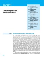
Definition 1.3.1 A set of gates is universal for classical computation if, for
any positive integers n, m, and function f : {0, 1}n → {0, 1}m , a circuit can be
constructed for computing f using only gates from that set.
A well-known example of a set of gates that is universal for classical computation is {nand, fanout}.1 If we restrict ourselves to reversible gates, we cannot
achieve universality with only one- and two-bit gates. The Toffoli gate is a reversible three-bit gate that has the effect of flipping the third bit, if and only
if the first two bits are both in state 1 (and does nothing otherwise). The set
consisting of just the Toffoli gate is universal for classical computation.2
In Section 1.2, we extended the definition of the Turing machine and defined
the probabilistic Turing machine. The probabilistic Turing machine is obtained
by equipping the Turing machine with a ‘coin-flipper’ capable of generating a
random binary value in a single time-step. (There are other equivalent ways of
formally defining a probabilistic Turing machine.) We mentioned that it is an
open question whether a probabilistic Turing machine is more powerful than a
deterministic Turing machine; there are some problems that we do not know how
to solve on a deterministic Turing machine but we know how to solve efficiently
on a probabilistic Turing machine. We can define a model of probabilistic circuits

similarly by allowing our circuits to use a ‘coin-flipping gate’, which is a gate that
acts on a single bit, and outputs a random binary value for that bit (independent
of the value of the input bit).
When we considered Turing machines in Section 1.2, we saw that the complexity
of a computation could be specified in terms of the amount of time or space the
machine uses to complete the computation. For the circuit model of computation
one natural measure of complexity is the number of gates used in the circuit Cn .
Another is the depth of the circuit. If we visualize the circuit as being divided
1 The NAND gate computes the negation of the logical AND function, and the FANOUT
gate outputs two copies of a single input wire.
2 For the Toffoli gate to be universal we need the ability to add ancillary bits to the circuit
that can be initialized to either 0 or 1 as required.

TEAM LinG


8

INTRODUCTION AND BACKGROUND

Fig. 1.2 A circuit of depth 5, space (width) 4, and having a total of 8 gates.

into a sequence of discrete time-slices, where the application of a single gate
requires a single time-slice, the depth of a circuit is its total number of timeslices. Note that this is not necessarily the same as the total number of gates in
the circuit, since gates that act on disjoint bits can often be applied in parallel
(e.g. a pair of gates could be applied to the bits on two different wires during
the same time-slice). A third measure of complexity for a circuit is analogous to
space for a Turing machine. This is the total number of bits, or ‘wires’ in the
circuit, sometimes called the width or space of the circuit. These measures of
circuit complexity are illustrated in Figure 1.2.

1.4

A Linear Algebra Formulation of the Circuit Model

In this section we formulate the circuit model of computation in terms of vectors and matrices. This is not a common approach taken for classical computer
science, but it does make the transition to the standard formulation of quantum computers much more direct. It will also help distinguish the new notations
used in quantum information from the new concepts. The ideas and terminology
presented here will be generalized and recur throughout this book.
Suppose you are given a description of a circuit (e.g. in a diagram like Figure 1.1),
and a specification of some input bit values. If you were asked to predict the
output of the circuit, the approach you would likely take would be to trace
through the circuit from left to right, updating the values of the bits stored on
each of the wires after each gate. In other words, you are following the ‘state’ of
the bits on the wires as they progress through the circuit. For a given point in
the circuit, we will often refer to the state of the bits on the wires at that point
in the circuit simply as the ‘state of the computer’ at that point.
The state associated with a given point in a deterministic (non-probabilistic)
circuit can be specified by listing the values of the bits on each of the wires
in the circuit. The ‘state’ of any particular wire at a given point in a circuit,
of course, is just the value of the bit on that wire (0 or 1). For a probabilistic
circuit, however, this simple description is not enough.
Consider a single bit that is in state 0 with probability p0 and in state 1 with
probability p1 . We can summarize this information by a 2-dimensional vector of
probabilities

TEAM LinG


A LINEAR ALGEBRA FORMULATION OF THE CIRCUIT MODEL

p0
.
p1

9

(1.4.1)

Note that this description can also be used for deterministic circuits. A wire in
a deterministic circuit whose state is 0 could be specified by the probabilities
p0 = 1 and p1 = 0, and the corresponding vector
1
.
0

(1.4.2)

Similarly, a wire in state 1 could be represented by the probabilities p0 = 0,
p1 = 1, and the vector
0
.
(1.4.3)
1
Since we have chosen to represent the states of wires (and collections of wires)
in a circuit by vectors, we would like to be able to represent gates in the circuit
by operators that act on the state vectors appropriately. The operators are conveniently described by matrices. Consider the logical not gate. We would like to
define an operator (matrix) that behaves on state vectors in a manner consistent
with the behaviour of the not gate. If we know a wire is in state 0 (so p0 = 1),
the not gate maps it to state 1 (so p1 = 1), and vice versa. In terms of the

vector representations of these states, we have
not

1
0

=

0
,
1

not

0
1

=

1
.
0

(1.4.4)

This implies that we can represent the not vector by the matrix
not ≡

01
.

10

(1.4.5)

To ‘apply’ the gate to a wire in a given state, we multiply the corresponding
state vector on the left by the matrix representation of the gate:
not

p0
p1

=

01
10

p1
.
p0

(1.4.6)

Suppose we want to describe the state associated with a given point in a probabilistic circuit having two wires. Suppose the state of the first wire at the given
point is 0 with probability p0 and 1 with probability p1 . Suppose the state of the
second wire at the given point is 0 with probability q0 and 1 with probability q1 .
The four possibilities for the combined state of both wires at the given point are
{00,01,10,11} (where the binary string ij indicates that the first wire is in state
i and the second wire in state j). The probabilities associated with each of these

TEAM LinG

10

INTRODUCTION AND BACKGROUND

four states are obtained by multiplying the corresponding probabilities for each
of the four states:
prob(ij) = pi qj .

(1.4.7)

This means that the combined state of both wires can be described by the
4-dimensional vector of probabilities
⎞
p 0 q0
⎜ p0 q 1 ⎟
⎟
⎜
⎝ p1 q 0 ⎠ .
p1 q 1
⎛

(1.4.8)

As we will see in Section 2.6, this vector is the tensor product of the 2-dimensional
vectors for the states of the first and second wires separately:
⎞
⎛
p0 q0

⎜p0 q1 ⎟
⎟
⎜
⎝p1 q0 ⎠ =
p1 q 1

p0
p1

⊗

q0
.
q1

(1.4.9)

Tensor products (which will be defined more generally in Section 2.6) arise naturally when we consider probabilistic systems composed of two or more subsystems.
We can also represent gates acting on more than one wire. For example, the
controlled-not gate, denoted cnot. This is a gate that acts on two bits, labelled
the control bit and the target bit. The action of the gate is to apply the not
operation to the target if the control bit is 0, and do nothing otherwise (the
control bit is always unaffected by the cnot gate). Equivalently, if the state of
the control bit is c, and the target bit is in state t the cnot gate maps the target
bit to t ⊕ c (where ‘⊕’ represents the logical exclusive-or operation, or addition
modulo 2). The cnot gate is illustrated in Figure 1.3.
The cnot gate can be represented by the matrix
⎡
1
⎢0

cnot ≡ ⎢
⎣0
0

0
1
0
0

0
0
0
1

⎤
0
0⎥
⎥.
1⎦
0

(1.4.10)

Fig. 1.3 The reversible cnot gate flips the value of the target bit t if and only if the
control bit c has value 1.

TEAM LinG


A LINEAR ALGEBRA FORMULATION OF THE CIRCUIT MODEL

11

Consider, for example, a pair of wires such that the first wire is in state 1 and
the second in state 0. This means that the 4-dimensional vector describing the
combined state of the pair of wires is
⎛ ⎞
0
⎜0⎟
⎜ ⎟.
(1.4.11)
⎝1⎠
0
Suppose we apply to the cnot gate to this pair of wires, with the first wire as the
control bit, and the second as the target bit. From the description of the cnot
gate, we expect the result should be that the control bit (first wire) remains in
state 1, and the target bit (second wire) flips to state 1. That is, we expect the
resulting state vector to be
⎛ ⎞
0
⎜0⎟
⎜ ⎟.
(1.4.12)
⎝0⎠
1
We can check that the matrix defined above for cnot does what we expect:
⎛ ⎞ ⎡
⎤⎛ ⎞ ⎛ ⎞
0
1000

0
0
⎜0⎟ ⎢0 1 0 0⎥ ⎜0⎟ ⎜0⎟
⎟ ⎢
⎥⎜ ⎟ ⎜ ⎟
cnot ⎜
(1.4.13)
⎝1⎠ ≡ ⎣0 0 0 1⎦ ⎝1⎠ = ⎝0⎠ .
0
0010
0
1
It is also interesting to note that if the first bit is in the state
⎛1⎞
⎜2⎟
⎝ ⎠
1
2
and the second bit is in the state
1
0
then applying the cnot will create the state
⎛1⎞
⎜2⎟
⎜ ⎟
⎜0 ⎟
⎜ ⎟.
⎜0 ⎟
⎝ ⎠
1

2
This state cannot be factorized into the tensor product of two independent probabilistic bits. The states of two such bits are correlated.

TEAM LinG


12

INTRODUCTION AND BACKGROUND

We have given a brief overview of the circuit model of computation, and presented
a convenient formulation for it in terms of matrices and vectors. The circuit model
and its formulation in terms of linear algebra will be generalized to describe
quantum computers in Chapter 4.

1.5

Reversible Computation

The theory of quantum computing is related to a theory of reversible computing.
A computation is reversible if it is always possible to uniquely recover the input,
given the output. For example, the not operation is reversible, because if the
output bit is 0, you know the input bit must have been 1, and vice versa. On
the other hand, the and operation is not reversible (see Figure 1.4).
As we now describe, any (generally irreversible) computation can be transformed
into a reversible computation. This is easy to see for the circuit model of computation. Each gate in a finite family of gates can be made reversible by adding some
additional input and output wires if necessary. For example, the and gate can be
made reversible by adding an additional input wire and two additional output
wires (see Figure 1.5). Note that additional information necessary to reverse the
operation is now kept and accounted for. Whereas in any physical implementation of a logically irreversible computation, the information that would allow

one to reverse it is somehow discarded or absorbed into the environment.

Fig. 1.4 The not and and gates. Note that the not gate is reversible while the and
gate is not.

Fig. 1.5 The reversible and gate keeps a copy of the inputs and adds the and of x0
and x1 (denoted x1 ∧ x2 ) to the value in the additional input bit. Note that by fixing
the additional input bit to 0 and discarding the copies of the x0 and x1 we can simulate
the non-reversible and gate.

TEAM LinG


REVERSIBLE COMPUTATION

13

Note that the reversible and gate which is in fact the Toffoli gate defined in
the previous section, is a generalization of the cnot gate (the cnot gate is
reversible), where there are two bits controlling whether the not is applied to
the third bit.
By simply replacing all the irreversible components with their reversible counterparts, we get a reversible version of the circuit. If we start with the output,
and run the circuit backwards (replacing each gate by its inverse), we obtain the
input again. The reversible version might introduce some constant number of
additional wires for each gate. Thus, if we have an irreversible circuit with depth
T and space S, we can easily construct a reversible version that uses a total of
O(S + ST ) space and depth T . Furthermore, the additional ‘junk’ information
generated by making each gate reversible can also be erased at the end of the
computation by first copying the output, and then running the reversible circuit
in reverse to obtain the starting state again. Of course, the copying has to be

done in a reversible manner, which means that we cannot simply overwrite the
value initially in the copy register. The reversible copying can be achieved by a
sequence of cnot gates, which xor the value being copied with the value initially in the copy register. By setting the bits in the copy register initially to 0,
we achieved the desired effect. This reversible scheme3 for computing a function
f is illustrated in Figure 1.6.

Exercise 1.5.1 A sequence of n cnot gates with the target bits all initialized to 0 is
the simplest way to copy an n-bit string y stored in the control bits. However, more
sophisticated copy operations are also possible, such as a circuit that treats a string
y as the binary representation of the integer y1 + 2y2 + 4y3 + · · · 2n−1 yn and adds y
modulo 2n to the copy register (modular arithmetic is defined in Section 7.3.2).
Describe a reversible 4-bit circuit that adds modulo 4 the integer y ∈ {0, 1, 2, 3} represented in binary in the first two bits to the integer z represented in binary in the last
two bits.

If we suppress the ‘temporary’ registers that are 0 both before and after the
computation, the reversible circuit effectively computes
(x1 , x2 , x3 ), (c1 , c2 , c3 ) −→ (x1 , x2 , x3 ), (c1 ⊕ y1 , c2 ⊕ y2 , c3 ⊕ y3 ),

(1.5.1)

where f (x1 , x2 , x3 ) = (y1 , y2 , y3 ). In general, given an implementation (not
necessarily reversible) of a function f , we can easily describe a reversible
implementation of the form
(x, c) −→ (x, c ⊕ f (x))
3 In general, reversible circuits for computing a function f do not need to be of this form,
and might require much fewer than twice the number of gates as a non-reversible circuit for
implementing f .

TEAM LinG

14

INTRODUCTION AND BACKGROUND

Input

Output

Workspace

Copy

Fig. 1.6 A circuit for reversibly computing f (x). Start with the input. Compute f (x)
using reversible logic, possibly generating some extra ‘junk’ bits j1 and j2 . The block
labelled Cf represents a circuit composed of reversible gates. Then copy the output
y = f (x) to another register. Finally run the circuit for Cf backwards (replacing each
gate by its inverse gate) to erase the contents of the output and workspace registers.
Note we write the operation of the backwards circuit by Cf−1 .

with modest overhead. There are more sophisticated techniques that can often be
applied to achieve reversible circuits with different time and space bounds than
described above. The approach we have described is intended to demonstrate that
in principle we can always find some reversible circuit for any given computation.
In classical computation, one could choose to be more environmentally friendly
and uncompute redundant or junk information, and reuse the cleared-up memory
for another computation. However, simply discarding the redundant information
does not actually affect the outcome of the computation. In quantum computation however, discarding information that is correlated to the bits you keep can
drastically change the outcome of a computation. For this reason, the theory of
reversible computation plays an important role in the development of quantum

algorithms. In a manner very similar to the classical case, reversible quantum
operations can efficiently simulate non-reversible quantum operations (and sometimes vice versa) so we generally focus attention on reversible quantum gates.
However, for the purposes of implementation or algorithm design, this is not always necessary (e.g. one can cleverly configure special families of non-reversible
gates to efficiently simulate reversible ones).

Example 1.5.1 As pointed out in Section 1.3, the computing model corresponding
to uniform families of acyclic reversible circuits can efficiently simulate any standard
model of classical computation. This section shows how any function that we know how
to efficiently compute on a classical computer has a uniform family of acyclic reversible
circuits that implements the function reversibly as illustrated in Equation 1.5.1.
Consider, for example, the arcsin function which maps [0, 1] → [0, π2 ] so that
sin(arcsin(x)) = x for any x ∈ [0, 1]. Since one can efficiently compute n-bit

TEAM LinG


A PREVIEW OF QUANTUM PHYSICS

15

D

P

Beam splitter

Fig. 1.7 Experimental setup with one beam splitter.
approximations of the arcsin function on a classical computer (e.g., using its Taylor
expansion), then there is a uniform family of acyclic reversible circuits, ARCSINn,m ,
of size polynomial in n and m, that implement the function arcsinn,m : {0, 1}n →

{0, 1}m which approximately computes the arcsin function in the following way. If
y = arcsinn,m (x), then
1
x
πy
arcsin n − m+1 < m .
2
2
2
The reversible circuit effectively computes
(x1 , x2 , . . . , xn ), (c1 , c2 , c3 , . . . , cm ) −→ (x1 , x2 , . . . , xn ), (c1 ⊕ y1 , c2 ⊕ y2 , . . . , cm ⊕ ym )
(1.5.2)
where y = y1 y2 . . . yn .

1.6

A Preview of Quantum Physics

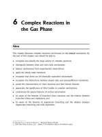
Here we describe an experimental set-up that cannot be described in a natural
way by classical physics, but has a simple quantum explanation. The point we
wish to make through this example is that the description of the universe given
by quantum mechanics differs in fundamental ways from the classical description.
Further, the quantum description is often at odds with our intuition, which has
evolved according to observations of macroscopic phenomena which are, to an
extremely good approximation, classical.
Suppose we have an experimental set-up consisting of a photon source, a beam
splitter (which was once implemented using a half-silvered mirror), and a pair
of photon detectors. The set-up is illustrated in Figure 1.7.
Suppose we send a series of individual photons4 along a path from the photon
source towards the beam splitter. We observe the photon arriving at the detector

on the right on the beam splitter half of the time, and arriving at the detector
above the beam splitter half of the time, as illustrated in Figure 1.8. The simplest
way to explain this behaviour in a theory of physics is to model the beam splitter
as effectively flipping a fair coin, and choosing whether to transmit or reflect the
4 When we reduce the intensity of a light source we observe that it actualy comes out in
discrete “chunks”, much like a faint beam of matter comes out one atom at a time. These
discrete quanta of light are called “photons”.

TEAM LinG