A study of the effect of molecular and aerosol conditions in the atmosphere on air fluorescence measurements at the pierre auger observatory
Bạn đang xem bản rút gọn của tài liệu. Xem và tải ngay bản đầy đủ của tài liệu tại đây (1.96 MB, 47 trang )
arXiv:1002.0366v1 [astro-ph.IM] 1 Feb 2010
A Study of the Effect of
Molecular and Aerosol Conditions in the Atmosphere
on Air Fluorescence Measurements at the
Pierre Auger Observatory
The Pierre Auger Collaboration
J. Abraham8 , P. Abreu71 , M. Aglietta54 , C. Aguirre12 , E.J. Ahn87 ,
D. Allard31 , I. Allekotte1 , J. Allen90 , J. Alvarez-Mu˜
niz78 , M. Ambrosio48 ,
104
71
53
L. Anchordoqui , S. Andringa , A. Anzalone , C. Aramo48 , E. Arganda75 ,
K. Arisaka95 , F. Arqueros75 , T. Asch38 , H. Asorey1 , P. Assis71 , J. Aublin33 ,
M. Ave37, 96 , G. Avila10 , T. Băacker42, D. Badagnani6 , K.B. Barber11 ,
A.F. Barbosa14, S.L.C. Barroso20, B. Baughman92 , P. Bauleo85 , J.J. Beatty92 ,
T. Beau31 , B.R. Becker101 , K.H. Becker36 , A. Bell´etoile34 , J.A. Bellido11 ,
S. BenZvi103 , C. Berat34 , X. Bertou1 , P.L. Biermann39 , P. Billoir33 ,
O. Blanch-Bigas33, F. Blanco75 , C. Bleve47 , H. Blă
umer41, 37 ,
96, 27
49
33
M. Boh´
aˇcov´
a
, D. Boncioli , C. Bonifazi , R. Bonino54 , N. Borodai69 ,
85
J. Brack , P. Brogueira71, W.C. Brown86 , R. Bruijn81 , P. Buchholz42 ,
A. Bueno77 , R.E. Burton83 , N.G. Busca31 , K.S. Caballero-Mora41,
L. Caramete39 , R. Caruso50 , A. Castellina54 , O. Catalano53 , L. Cazon96 ,
R. Cester51 , J. Chauvin34 , A. Chiavassa54 , J.A. Chinellato18 , A. Chou87, 90 ,
J. Chudoba27 , J. Chye89 d , R.W. Clay11 , E. Colombo2 , R. Concei¸c˜ao71 ,
F. Contreras9, H. Cook81 , J. Coppens65, 67 , A. Cordier32 , U. Cotti63 ,
S. Coutu93 , C.E. Covault83 , A. Creusot73 , A. Criss93 , J. Cronin96 ,
A. Curutiu39 , S. Dagoret-Campagne32, R. Dallier35 , K. Daumiller37 ,
B.R. Dawson11 , R.M. de Almeida18 , M. De Domenico50 , C. De Donato46 ,
S.J. de Jong65 , G. De La Vega8 , W.J.M. de Mello Junior18 , J.R.T. de Mello
Neto23 , I. De Mitri47 , V. de Souza16 , K.D. de Vries66 , G. Decerprit31 , L. del
Peral76, O. Deligny30 , A. Della Selva48 , C. Delle Fratte49 , H. Dembinski40 ,
C. Di Giulio49 , J.C. Diaz89 , P.N. Diep105 , C. Dobrigkeit 18 , J.C. D’Olivo64 ,
P.N. Dong105 , A. Dorofeev85 , J.C. dos Anjos14 , M.T. Dova6 , D. D’Urso48 ,
I. Dutan39 , M.A. DuVernois98 , J. Ebr27 , R. Engel37 , M. Erdmann40 ,
C.O. Escobar18, A. Etchegoyen2, P. Facal San Luis96, 78 , H. Falcke65, 68 ,
G. Farrar90, A.C. Fauth18 , N. Fazzini87 , F. Ferrer83 , A. Ferrero2 , B. Fick89 ,
A. Filevich2 , A. Filipˇciˇc72, 73 , I. Fleck42 , S. Fliescher40 , C.E. Fracchiolla85,
E.D. Fraenkel66 , W. Fulgione54 , R.F. Gamarra2 , S. Gambetta44 , B. Garc´ıa8,
D. Garc´ıa G´
amez77 , D. Garcia-Pinto75, X. Garrido37, 32 , G. Gelmini95 ,
H. Gemmeke38 , P.L. Ghia30, 54 , U. Giaccari47 , M. Giller70 , H. Glass87 ,
L.M. Goggin104 , M.S. Gold101 , G. Golup1 , F. Gomez Albarracin6 , M. G´omez
Berisso1 , P. Gon¸calves71 , D. Gonzalez41 , J.G. Gonzalez77, 88 , D. G´ora41, 69 ,
A. Gorgi54 , P. Gouffon17 , S.R. Gozzini81 , E. Grashorn92 , S. Grebe65 ,
M. Grigat40 , A.F. Grillo55 , Y. Guardincerri4 , F. Guarino48 , G.P. Guedes19 ,
J. Guti´errez76 , J.D. Hague101 , V. Halenka28 , P. Hansen6 , D. Harari1 ,
S. Harmsma66, 67 , J.L. Harton85 , A. Haungs37 , M.D. Healy95 , T. Hebbeker40 ,
G. Hebrero76 , D. Heck37 , C. Hojvat87 , V.C. Holmes11 , P. Homola69 ,
Preprint submitted to Astropart. Phys.
February 1, 2010
J.R. Hă
orandel65 , A. Horneer65 , M. Hrabovsk
y28, 27 , T. Huege37 ,
73
45
50
M. Hussain , M. Iarlori , A. Insolia , F. Ionita96 , A. Italiano50 ,
S. Jiraskova65, M. Kaducak87, K.H. Kampert36 , T. Karova27, P. Kasper87 ,
B. K´egl32, B. Keilhauer37 , J. Kelley65 , E. Kemp18 , R.M. Kieckhafer89 ,
H.O. Klages37, M. Kleifges38 , J. Kleinfeller37 , R. Knapik85 , J. Knapp81 ,
D.-H. Koang34, A. Krieger2, O. Krăomer38 , D. Kruppke-Hansen36, F. Kuehn87 ,
D. Kuempel36 , K. Kulbartz43 , N. Kunka38 , A. Kusenko95 , G. La Rosa53 ,
C. Lachaud31 , B.L. Lago23 , P. Lautridou35 , M.S.A.B. Le˜ao22 , D. Lebrun34 ,
P. Lebrun87 , J. Lee95 , M.A. Leigui de Oliveira22, A. Lemiere30 ,
A. Letessier-Selvon33, I. Lhenry-Yvon30 , R. Lopez59 , A. Lopez Agă
uera78 ,
32
77
54
41
K. Louedec , J. Lozano Bahilo , A. Lucero , M. Ludwig , H. Lyberis30 ,
M.C. Maccarone53, C. Macolino45 , S. Maldera54 , D. Mandat27 , P. Mantsch87 ,
A.G. Mariazzi6 , I.C. Maris41 , H.R. Marquez Falcon63 , G. Marsella52 ,
D. Martello47 , O. Mart´ınez Bravo59, H.J. Mathes37 , J. Matthews88, 94 ,
J.A.J. Matthews101 , G. Matthiae49 , D. Maurizio51 , P.O. Mazur87 ,
M. McEwen76 , R.R. McNeil88 , G. Medina-Tanco64 , M. Melissas41 , D. Melo51 ,
E. Menichetti51 , A. Menshikov38 , C. Meurer40 , M.I. Micheletti2 , W. Miller101 ,
L. Miramonti46 , S. Mollerach1, M. Monasor75, D. Monnier Ragaigne32 ,
F. Montanet34 , B. Morales64 , C. Morello54 , J.C. Moreno6 , C. Morris92 ,
M. Mostaf´
a85 , C.A. Moura48 , S. Mueller37 , M.A. Muller18 , R. Mussa51 ,
G. Navarra54, J.L. Navarro77, S. Navas77 , P. Necesal27 , L. Nellen64 ,
C. Newman-Holmes87 , P.T. Nhung105 , N. Nierstenhoefer36 , D. Nitz89 ,
D. Nosek26 , L. Nozka27 , M. Nyklicek27 , J. Oehlschlăager37, A. Olinto96 ,
P. Oliva36 , V.M. Olmos-Gilbaja78, M. Ortiz75 , N. Pacheco76 , D. Pakk
Selmi-Dei18 , M. Palatka27 , J. Pallotta3 , N. Palmieri41, G. Parente78 ,
E. Parizot31, S. Parlati55, R.D. Parsons81, S. Pastor74 , T. Paul91 ,
V. Pavlidou96 c , K. Payet34 , M. Pech27 , J. P¸ekala69 , I.M. Pepe21 , L. Perrone52,
R. Pesce44 , E. Petermann100 , S. Petrera45, P. Petrinca49 , A. Petrolini44 ,
Y. Petrov85, J. Petrovic67 , C. Pfendner103 , R. Piegaia4, T. Pierog37 ,
M. Pimenta71 , V. Pirronello50, M. Platino2 , V.H. Ponce1 , M. Pontz42 ,
P. Privitera96 , M. Prouza27 , E.J. Quel3 , J. Rautenberg36 , O. Ravel35 ,
D. Ravignani2 , A. Redondo76 , B. Revenu35 , F.A.S. Rezende14 , J. Ridky27 ,
S. Riggi50 , M. Risse36 , C. Rivi`ere34 , V. Rizi45 , C. Robledo59 , G. Rodriguez49 ,
J. Rodriguez Martino50 , J. Rodriguez Rojo9 , I. Rodriguez-Cabo78 ,
M.D. Rodr´ıguez-Fr´ıas76, G. Ros75, 76 , J. Rosado75 , T. Rossler28, M. Roth37 ,
B. Rouill´e-d’Orfeuil31, E. Roulet1 , A.C. Rovero7, F. Salamida45 ,
H. Salazar59 b , G. Salina49 , F. S´anchez64 , M. Santander9 , C.E. Santo71 ,
E. Santos71 , E.M. Santos23 , F. Sarazin84 , S. Sarkar79 , R. Sato9 , N. Scharf40 ,
V. Scherini36 , H. Schieler37 , P. Schiffer40 , A. Schmidt38 , F. Schmidt96 ,
T. Schmidt41 , O. Scholten66 , H. Schoorlemmer65, J. Schovancova27,
P. Schov´
anek27 , F. Schroeder37 , S. Schulte40 , F. Schă
ussler37 , D. Schuster84 ,
6
50
53
S.J. Sciutto , M. Scuderi , A. Segreto , D. Semikoz31 , M. Settimo47 ,
70
´
R.C. Shellard14, 15 , I. Sidelnik2 , B.B. Siffert23 , G. Sigl43 , A. Smialkowski
,
27
100
93
11
82, 87
ˇ
R. Sm´ıda , G.R. Snow , P. Sommers , J. Sorokin , H. Spinka
,
R. Squartini9 , E. Strazzeri53, 32 , A. Stutz34 , F. Suarez2 , T. Suomijăarvi30 ,
A.D. Supanitsky64 , M.S. Sutherland92 , J. Swain91 , Z. Szadkowski70,
2
A. Tamashiro7, A. Tamburro41 , T. Tarutina6 , O. Ta¸sc˘au36 , R. Tcaciuc42 ,
D. Tcherniakhovski38, D. Tegolo58 , N.T. Thao105 , D. Thomas85 , R. Ticona13 ,
J. Tiffenberg4 , C. Timmermans67, 65 , W. Tkaczyk70 , C.J. Todero Peixoto22 ,
B. Tom´e71 , A. Tonachini51 , I. Torres59, P. Travnicek27 , D.B. Tridapalli17 ,
G. Tristram31 , E. Trovato50 , M. Tueros6 , R. Ulrich37 , M. Unger37 ,
M. Urban32 , J.F. Vald´es Galicia64 , I. Vali˜
no37 , L. Valore48 , A.M. van den
66
75
78
Berg , J.R. V´
azquez , R.A. V´azquez , D. Veberiˇc73, 72 , A. Velarde13 ,
96
T. Venters , V. Verzi49 , M. Videla8 , L. Villase˜
nor63 , S. Vorobiov73,
87 ‡
6
11
L. Voyvodic
, H. Wahlberg , P. Wahrlich , O. Wainberg2 , D. Warner85 ,
A.A. Watson81 , S. Westerhoff103 , B.J. Whelan11 , G. Wieczorek70 ,
L. Wiencke84 , B. Wilczy´
nska69 , H. Wilczy´
nski69 , T. Winchen40 ,
11
32
2
M.G. Winnick , H. Wu , B. Wundheiler , T. Yamamoto96 a , P. Younk85 ,
G. Yuan88 , A. Yushkov48 , E. Zas78 , D. Zavrtanik73, 72 , M. Zavrtanik72, 73 ,
I. Zaw90 , A. Zepeda60 , M. Ziolkowski42
1
Centro At´
omico Bariloche and Instituto Balseiro (CNEAUNCuyo-CONICET), San Carlos de Bariloche, Argentina
2
Centro At´
omico Constituyentes (Comisi´
on Nacional de Energ´ıa
At´
omica/CONICET/UTN-FRBA), Buenos Aires, Argentina
3
Centro de Investigaciones en L´aseres y Aplicaciones, CITEFA and
CONICET, Argentina
4
Departamento de F´ısica, FCEyN, Universidad de Buenos Aires y CONICET,
Argentina
6
IFLP, Universidad Nacional de La Plata and CONICET, La Plata, Argentina
7
Instituto de Astronom´ıa y F´ısica del Espacio (CONICET), Buenos Aires,
Argentina
8
National Technological University, Faculty Mendoza (CONICET/CNEA),
Mendoza, Argentina
9
Pierre Auger Southern Observatory, Malargă
ue, Argentina
10
Pierre Auger Southern Observatory and Comision Nacional de Energa
At
omica, Malargă
ue, Argentina
11
University of Adelaide, Adelaide, S.A., Australia
12
Universidad Catolica de Bolivia, La Paz, Bolivia
13
Universidad Mayor de San Andr´es, Bolivia
14
Centro Brasileiro de Pesquisas Fisicas, Rio de Janeiro, RJ, Brazil
15
Pontif´ıcia Universidade Cat´olica, Rio de Janeiro, RJ, Brazil
16
Universidade de S˜
ao Paulo, Instituto de F´ısica, S˜ao Carlos, SP, Brazil
17
Universidade de S˜
ao Paulo, Instituto de F´ısica, S˜ao Paulo, SP, Brazil
18
Universidade Estadual de Campinas, IFGW, Campinas, SP, Brazil
19
Universidade Estadual de Feira de Santana, Brazil
20
Universidade Estadual do Sudoeste da Bahia, Vitoria da Conquista, BA,
Brazil
21
Universidade Federal da Bahia, Salvador, BA, Brazil
22
Universidade Federal do ABC, Santo Andr´e, SP, Brazil
23
Universidade Federal do Rio de Janeiro, Instituto de F´ısica, Rio de Janeiro,
RJ, Brazil
26
Charles University, Faculty of Mathematics and Physics, Institute of
3
Particle and Nuclear Physics, Prague, Czech Republic
Institute of Physics of the Academy of Sciences of the Czech Republic,
Prague, Czech Republic
28
Palack´
y University, Olomouc, Czech Republic
30
Institut de Physique Nucl´eaire d’Orsay (IPNO), Universit´e Paris 11,
CNRS-IN2P3, Orsay, France
31
Laboratoire AstroParticule et Cosmologie (APC), Universit´e Paris 7,
CNRS-IN2P3, Paris, France
32
Laboratoire de l’Acc´el´erateur Lin´eaire (LAL), Universit´e Paris 11,
CNRS-IN2P3, Orsay, France
33
Laboratoire de Physique Nucl´eaire et de Hautes Energies (LPNHE),
Universit´es Paris 6 et Paris 7, CNRS-IN2P3, Paris, France
34
Laboratoire de Physique Subatomique et de Cosmologie (LPSC), Universit´e
Joseph Fourier, INPG, CNRS-IN2P3, Grenoble, France
35
SUBATECH, CNRS-IN2P3, Nantes, France
36
Bergische Universităat Wuppertal, Wuppertal, Germany
37
Forschungszentrum Karlsruhe, Institut fă
ur Kernphysik, Karlsruhe, Germany
38
Forschungszentrum Karlsruhe, Institut fă
ur Prozessdatenverarbeitung und
Elektronik, Karlsruhe, Germany
39
Max-Planck-Institut fă
ur Radioastronomie, Bonn, Germany
40
RWTH Aachen University, III. Physikalisches Institut A, Aachen, Germany
41
Universită
at Karlsruhe (TH), Institut fă
ur Experimentelle Kernphysik
(IEKP), Karlsruhe, Germany
42
Universităat Siegen, Siegen, Germany
43
Universităat Hamburg, Hamburg, Germany
44
Dipartimento di Fisica dellUniversit`a and INFN, Genova, Italy
45
Universit`
a dell’Aquila and INFN, L’Aquila, Italy
46
Universit`
a di Milano and Sezione INFN, Milan, Italy
47
Dipartimento di Fisica dell’Universit`a del Salento and Sezione INFN, Lecce,
Italy
48
Universit`
a di Napoli “Federico II” and Sezione INFN, Napoli, Italy
49
Universit`
a di Roma II “Tor Vergata” and Sezione INFN, Roma, Italy
50
Universit`
a di Catania and Sezione INFN, Catania, Italy
51
Universit`
a di Torino and Sezione INFN, Torino, Italy
52
Dipartimento di Ingegneria dell’Innovazione dell’Universit`a del Salento and
Sezione INFN, Lecce, Italy
53
Istituto di Astrofisica Spaziale e Fisica Cosmica di Palermo (INAF),
Palermo, Italy
54
Istituto di Fisica dello Spazio Interplanetario (INAF), Universit`a di Torino
and Sezione INFN, Torino, Italy
55
INFN, Laboratori Nazionali del Gran Sasso, Assergi (L’Aquila), Italy
58
Universit`
a di Palermo and Sezione INFN, Catania, Italy
59
Benem´erita Universidad Aut´onoma de Puebla, Puebla, Mexico
60
Centro de Investigaci´on y de Estudios Avanzados del IPN (CINVESTAV),
M´exico, D.F., Mexico
61
Instituto Nacional de Astrofisica, Optica y Electronica, Tonantzintla,
27
4
Puebla, Mexico
Universidad Michoacana de San Nicolas de Hidalgo, Morelia, Michoacan,
Mexico
64
Universidad Nacional Autonoma de Mexico, Mexico, D.F., Mexico
65
IMAPP, Radboud University, Nijmegen, Netherlands
66
Kernfysisch Versneller Instituut, University of Groningen, Groningen,
Netherlands
67
NIKHEF, Amsterdam, Netherlands
68
ASTRON, Dwingeloo, Netherlands
69
Institute of Nuclear Physics PAN, Krakow, Poland
70
University of L´od´z, L´od´z, Poland
71
LIP and Instituto Superior T´ecnico, Lisboa, Portugal
72
J. Stefan Institute, Ljubljana, Slovenia
73
Laboratory for Astroparticle Physics, University of Nova Gorica, Slovenia
74
Instituto de F´ısica Corpuscular, CSIC-Universitat de Val`encia, Valencia,
Spain
75
Universidad Complutense de Madrid, Madrid, Spain
76
Universidad de Alcal´
a, Alcal´
a de Henares (Madrid), Spain
77
Universidad de Granada & C.A.F.P.E., Granada, Spain
78
Universidad de Santiago de Compostela, Spain
79
Rudolf Peierls Centre for Theoretical Physics, University of Oxford, Oxford,
United Kingdom
81
School of Physics and Astronomy, University of Leeds, United Kingdom
82
Argonne National Laboratory, Argonne, IL, USA
83
Case Western Reserve University, Cleveland, OH, USA
84
Colorado School of Mines, Golden, CO, USA
85
Colorado State University, Fort Collins, CO, USA
86
Colorado State University, Pueblo, CO, USA
87
Fermilab, Batavia, IL, USA
88
Louisiana State University, Baton Rouge, LA, USA
89
Michigan Technological University, Houghton, MI, USA
90
New York University, New York, NY, USA
91
Northeastern University, Boston, MA, USA
92
Ohio State University, Columbus, OH, USA
93
Pennsylvania State University, University Park, PA, USA
94
Southern University, Baton Rouge, LA, USA
95
University of California, Los Angeles, CA, USA
96
University of Chicago, Enrico Fermi Institute, Chicago, IL, USA
98
University of Hawaii, Honolulu, HI, USA
100
University of Nebraska, Lincoln, NE, USA
101
University of New Mexico, Albuquerque, NM, USA
103
University of Wisconsin, Madison, WI, USA
104
University of Wisconsin, Milwaukee, WI, USA
105
Institute for Nuclear Science and Technology (INST), Hanoi, Vietnam
(‡) Deceased
(a) at Konan University, Kobe, Japan
63
5
(b) On leave of absence at the Instituto Nacional de Astrofisica, Optica y
Electronica
(c) at Caltech, Pasadena, USA
(d) at Hawaii Pacific University
Abstract
The air fluorescence detector of the Pierre Auger Observatory is designed to
perform calorimetric measurements of extensive air showers created by cosmic
rays of above 1018 eV. To correct these measurements for the effects introduced
by atmospheric fluctuations, the Observatory contains a group of monitoring
instruments to record atmospheric conditions across the detector site, an area
exceeding 3,000 km2 . The atmospheric data are used extensively in the
reconstruction of air showers, and are particularly important for the correct
determination of shower energies and the depths of shower maxima. This
paper contains a summary of the molecular and aerosol conditions measured
at the Pierre Auger Observatory since the start of regular operations in 2004,
and includes a discussion of the impact of these measurements on air shower
reconstructions. Between 1018 and 1020 eV, the systematic uncertainties due
to all atmospheric effects increase from 4% to 8% in measurements of shower
energy, and 4 g cm−2 to 8 g cm−2 in measurements of the shower maximum.
Key words: Cosmic rays, extensive air showers, air fluorescence method,
atmosphere, aerosols, lidar, bi-static lidar
6
1. Introduction
The Pierre Auger Observatory in Malargă
ue, Argentina (69 W, 35◦ S, 1400 m
a.s.l.) is a facility for the study of ultra-high energy cosmic rays. These
are primarily protons and nuclei with energies above 1018 eV. Due to the
extremely low flux of high-energy cosmic rays at Earth, the direct detection of
such particles is impractical; but when cosmic rays enter the atmosphere, they
produce extensive air showers of secondary particles. Using the atmosphere as
the detector volume, the air showers can be recorded and used to reconstruct
the energies, arrival directions, and nuclear mass composition of primary cosmic
ray particles. However, the constantly changing properties of the atmosphere
pose unique challenges for cosmic ray measurements.
In this paper, we describe the atmospheric monitoring data recorded at the
Pierre Auger Observatory and their effect on the reconstruction of air showers.
The paper is organized as follows: Section 2 contains a review of the observation
of air showers by their ultraviolet light emission, and includes a description of the
Pierre Auger Observatory and the issues of light production and transmission
that arise when using the atmosphere to make cosmic ray measurements.
The specifics of light attenuation by aerosols and molecules are described in
Section 3. An overview of local molecular measurements is given in Section 4,
and in Section 5 we discuss cloud-free aerosol measurements performed at
the Observatory. The impact of these atmospheric measurements on the
reconstruction of air showers is explored in Section 6. Cloud measurements
with infrared cameras and backscatter lidars are briefly described in Section 7.
Conclusions are given in Section 8.
2. Cosmic Ray Observations using Atmospheric Calorimetry
2.1. The Air Fluorescence Technique
The charged secondary particles in extensive air showers produce copious
amounts of ultraviolet light – of order 1010 photons per meter near the peak
of a 1019 eV shower. Some of this light is due to nitrogen fluorescence, in
which molecular nitrogen excited by a passing shower emits photons isotropically
into several dozen spectral bands between 300 and 420 nm. A much larger
fraction of the shower light is emitted as Cherenkov photons, which are strongly
beamed along the shower axis. With square-meter scale telescopes and sensitive
photodetectors, the UV emission from the highest energy air showers can be
observed at distances in excess of 30 km from the shower axis.
The flux of fluorescence photons from a given point on an air shower track
is proportional to dE/dX, the energy loss of the shower per unit slant depth
X of traversed atmosphere [1, 2]. The emitted light can be used to make a
calorimetric estimate of the energy of the primary cosmic ray [3, 4], after a
small correction for the “missing energy” not contained in the electromagnetic
component of the shower. Note that a large fraction of the light received from a
shower may be contaminated by Cherenkov photons. However, if the Cherenkov
7
fraction is carefully estimated, it can also be used to measure the longitudinal
development of a shower [4].
The fluorescence technique can also be used to determine cosmic ray
composition. The slant depth at which the energy deposition rate, dE/dX,
reaches its maximum value, denoted Xmax , is correlated with the mass of the
primary particle [5, 6]. Showers generated by light nuclei will, on average,
penetrate more deeply into the atmosphere than showers initiated by heavy
particles of the same energy, although the exact behavior is dependent on details
of hadronic interactions and must be inferred from Monte Carlo simulations. By
observing the UV light from air showers, it is possible to estimate the energies
of individual cosmic rays, as well as the average mass of a cosmic ray data set.
2.2. Challenges of Atmospheric Calorimetry
The atmosphere is responsible for producing light from air showers. Its
properties are also important for the transmission efficiency of light from the
shower to the air fluorescence detector. The atmosphere is variable, and so
measurements performed with the air fluorescence technique must be corrected
for changing conditions, which affect both light production and transmission.
For example, extensive balloon measurements conducted at the Pierre Auger
Observatory [7] and a study using radiosonde data from various geographic
locations [8] have shown that the altitude profile of the atmospheric depth,
X(h), typically varies by ∼ 5 g cm−2 from one night to the next. In extreme
cases, the depth can change by 20 g cm−2 on successive nights, which is similar
to the differences in depth between the seasons [9]. The largest variations are
comparable to the Xmax resolution of the Auger air fluorescence detector, and
could introduce significant biases into the determination of Xmax if not properly
measured. Moreover, changes in the bulk properties of the atmosphere such as
air pressure p, temperature T , and humidity u can have a significant effect on
the rate of nitrogen fluorescence emission [10], as well as light transmission.
In the lowest 15 km of the atmosphere where air shower measurements occur,
sub-µm to mm-sized aerosols also play an important role in modifying the light
transmission. Most aerosols are concentrated in a boundary layer that extends
about 1 km above the ground, and throughout most of the troposphere, the
ultraviolet extinction due to aerosols is typically several times smaller than the
extinction due to molecules [11, 12, 13]. However, the variations in aerosol
conditions have a greater effect on air shower measurements than variations in
p, T , and u, and during nights with significant haze, the light flux from distant
showers can be reduced by factors of 3 or more due to aerosol attenuation. The
vertical density profile of aerosols, as well as their size, shape, and composition,
vary quite strongly with location and in time, and depending on local particle
sources (dust, smoke, etc.) and sinks (wind and rain), the density of aerosols
can change substantially from hour to hour. If not properly measured, such
dynamic conditions can bias shower reconstructions.
8
2.3. The Pierre Auger Observatory
The Pierre Auger Observatory contains two cosmic ray detectors. The first
is a Surface Detector (SD) comprising 1600 water Cherenkov stations to observe
air shower particles that reach the ground [14]. The stations are arranged on a
triangular grid of 1.5 km spacing, and the full SD covers an area of 3,000 km2 .
The SD has a duty cycle of nearly 100%, allowing it to accumulate high-energy
statistics at a much higher rate than was possible at previous observatories.
Operating in concert with the SD is a Fluorescence Detector (FD) of 24
UV telescopes [15]. The telescopes are arranged to overlook the SD from four
buildings around the edge of the ground array. Each of the four FD buildings
contains six telescopes, and the total field of view at each site is 180◦ in azimuth
and 1.8◦ − 29.4◦ in elevation. The main component of a telescope is a spherical
mirror of area 11 m2 that directs collected light onto a camera of 440 hexagonal
photomultipliers (PMTs). One photomultiplier “pixel” views approximately
1.5◦ × 1.5◦ of the sky, and its output is digitized at 10 MHz. Hence, every PMT
camera can record the development of air showers with 100 ns time resolution.
The FD is only operated during dark and clear conditions, when the shower
UV signal is not overwhelmed by moonlight or blocked by low clouds or rain.
These limitations restrict the FD duty cycle to ∼ 10%− 15%, but unlike the SD,
the FD data provide calorimetric estimates of shower energies. Simultaneous SD
and FD measurements of air showers, known as hybrid observations, are used to
calibrate the absolute energy scale of the SD, reducing the need to calibrate the
SD with shower simulations. The hybrid operation also dramatically improves
the geometrical and longitudinal profile reconstruction of showers measured by
the FD, compared to showers observed by the FD alone [16, 17, 18, 19]. This
high-quality hybrid data set is used for all physics analyses based on the FD.
To remove the effect of atmospheric fluctuations that would otherwise impact
FD measurements, an extensive atmospheric monitoring program is carried out
at the Pierre Auger Observatory. A list of monitors and their locations relative
to the FD buildings and SD array are shown in fig. 1. Atmospheric conditions
at ground level are measured by a network of weather stations at each FD site
and in the center of the SD; these provide updates on ground-level conditions
every five minutes. In addition, regular meteorological radiosonde flights (one
or two per week) are used to measure the altitude profiles of atmospheric
pressure, temperature, and other bulk properties of the air. The weather station
monitoring and radiosonde flights are performed day or night, independent of
the FD data acquisition.
During the dark periods suitable for FD data-taking, hourly measurements of
aerosols are made using the FD telescopes, which record vertical UV laser tracks
produced by a Central Laser Facility (CLF) deployed on site since 2003 [20].
These measurements are augmented by data from lidar stations located near
each FD building [21], a Raman lidar at one FD site, and the eXtreme Laser
Facility (or XLF, named for its remote location) deployed in November 2008.
Two Aerosol Phase Function Monitors (APFs) are used to determine the aerosol
scattering properties of the atmosphere using collimated horizontal light beams
9
FD Loma Amarilla:
Lidar
IR Camera
Weather Station
FD Coihueco:
Lidar, APF
IR Camera
Weather Station
eXtreme Laser Facility
Balloon
Launch
Station
Central Laser Facility
Weather Station
FD Los Morados:
Lidar, APF
IR Camera
Weather Station
Malargue
FD Los Leones:
Lidar, Raman, HAM, FRAM
IR Camera
Weather Station
10 km
Figure 1: The Surface Detector stations and Fluorescence Detector sites of the Pierre Auger
Observatory. Also shown are the locations of Malargă
ue and the atmospheric monitoring
instruments operating at the Observatory (see text for details).
produced by Xenon flashers [22]. Two optical telescopes — the Horizontal
Attenuation Monitor (HAM) and the (F/ph)otometric Robotic Telescope
for Atmospheric Monitoring (FRAM) — record data used to determine the
wavelength dependence of the aerosol attenuation [23, 24]. Finally, clouds are
measured hourly by the lidar stations, and infrared cameras on the roof of each
FD building are used to record the cloud coverage in the FD field of view every
five minutes [25].
3. The Production of Light by the Shower and its Transmission
through the Atmosphere
Atmospheric conditions impact on both the production and transmission
of UV shower light recorded by the FD. The physical conditions of the
molecular atmosphere have several effects on fluorescence light production,
which we summarize in Section 3.1. We treat light transmission, outlined
in Section 3.2, primarily as a single-scattering process characterized by the
atmospheric optical depth (Sections 3.2.1 and 3.2.2) and scattering angular
dependence (Section 3.2.3). Multiple scattering corrections to atmospheric
transmission are discussed in Section 3.2.4.
3.1. The Effect of Weather on Light Production
The yields of light from the Cherenkov and fluorescence emission processes
depend on the physical conditions of the gaseous mixture of molecules in the
10
atmosphere. The production of Cherenkov light is the simpler of the two
cases, since the number of photons emitted per charged particle per meter per
wavelength interval depends only on the refractive index of the atmosphere
n(λ, p, T ). The dependence of this quantity on pressure, temperature, and
wavelength λ can be estimated analytically, and so the effect of weather on
the light yield from the Cherenkov process are relatively simple to incorporate
into air shower reconstructions.
The case of fluorescence light is more complex, not only because it is
necessary to consider additional weather effects on the light yield, but also
due to the fact that several of these effects can be determined only by difficult
experimental measurements (see [26, 27, 28, 29] and references in [30]).
One well-known effect of the weather on light production is the collisional
quenching of fluorescence emission, in which the radiative transitions of excited
nitrogen molecules are suppressed by molecular collisions. The rate of collisions
depends on pressure and temperature, and the form of this dependence can be
predicted by kinetic gas theory [1, 27]. However, the cross section for collisions
is itself a function of temperature, which introduces an additional term into the
p and T dependence of the yield. The temperature dependence of the cross
section cannot be predicted a priori, and must be determined with laboratory
measurements [31].
Water vapor in the atmosphere also contributes to collisional quenching, and
so the fluorescence yield has an additional dependence on the absolute humidity
of the atmosphere. This dependence must also be determined experimentally,
and its use as a correction in shower reconstructions using the fluorescence
technique requires regular measurements of the altitude profile of humidity. A
full discussion of these effects is beyond the scope of this paper, but detailed
descriptions are available in [2, 10, 32]. We will summarize the estimates of
their effect on shower energy and Xmax in Section 6.1.
3.2. The Effect of Weather on Light Transmission
The attenuation of light along a path through the atmosphere between a
light source and an observer can be expressed as a transmission coefficient T ,
which gives the fraction of light not absorbed or scattered along the path. If the
optical thickness (or optical depth) of the path is τ , then T is estimated using
the Beer-Lambert-Bouguer law:
T = e−τ .
(1)
The optical depth of the air is affected by the density and composition of
molecules and aerosols, and can be treated as the sum of molecular and aerosol
components: τ = τm + τa . The optical depth is a function of wavelength and
the orientation of a path within the atmosphere. However, if the atmospheric
region of interest is composed of horizontally uniform layers, then the full spatial
dependence of τ reduces to an altitude dependence, such that τ ≡ τ (h, λ). For
a slant path elevated at an angle ϕ above the horizon, the light transmission
11
along the path between the ground and height h is
T (h, λ, ϕ) = e−τ (h,λ)/ sin ϕ .
(2)
In an air fluorescence detector, a telescope recording isotropic fluorescence
emission of intensity I0 from a source of light along a shower track will observe
an intensity
∆Ω
I = I0 · Tm · Ta · (1 + H.O.) ·
,
(3)
4π
where ∆Ω is the solid angle subtended by the telescope diaphragm as seen from
the light source. The molecular and aerosol transmission factor Tm ·Ta primarily
represents single-scattering of photons out of the field of view of the telescope.
In the ultraviolet range used for air fluorescence measurements, the absorption
of light is much less important than scattering [11, 33], although there are
some exceptions discussed in Section 3.2.1. The term H.O. is a higher-order
correction to the Beer-Lambert-Bouguer law that accounts for the single and
multiple scattering of Cherenkov and fluorescence photons into the field of view.
To estimate the transmission factors and scattering corrections needed in
eq. (3), it is necessary to measure the vertical height profile and wavelength
dependence of the optical depth τ (h, λ), as well as the angular distribution of
light scattered from atmospheric particles, also known as the phase function
P (θ). For these quantities, the contributions due to molecules and aerosols are
considered separately.
3.2.1. The Optical Depth of Molecules
The probability per unit length that a photon will be scattered or absorbed
as it moves through the atmosphere is given by the total volume extinction
coefficient
αext (h, λ) = αabs (h, λ) + β(h, λ),
(4)
where αabs and β are the coefficients of absorption and scattering, respectively.
The vertical optical depth between a telescope at ground level and altitude h is
the integral of the atmospheric extinction along the path:
h
αext (h′ , λ)dh′ .
τ (h, λ) =
(5)
hgnd
Molecular extinction in the near UV is primarily an elastic scattering process,
since the Rayleigh scattering of light by molecular nitrogen (N2 ) and oxygen
(O2 ) dominates inelastic scattering and absorption [34]. For example, the
Raman scattering cross sections of N2 and O2 are approximately 10−30 cm−2
between 300 − 420 nm [35], much smaller than the Rayleigh scattering cross
section of air (∼ 10−27 cm−2 ) at these wavelengths [36]. Moreover, while O2 is
an important absorber in the deep UV, its absorption cross section is effectively
zero for wavelengths above 240 nm [33]. Ozone (O3 ) molecules absorb light in
the UV and visible bands, but O3 is mainly concentrated in a high-altitude layer
above the atmospheric volume used for air fluorescence measurements [33].
12
Therefore, for the purpose of air fluorescence detection, the total molecular
extinction αm
ext (h, λ) simply reduces to the scattering coefficient βm (h, λ).
At standard temperature and pressure, molecular scattering can be defined
analytically in terms of the Rayleigh scattering cross section [36, 37]:
STP
βm
(h, λ)
24π 3
≡ βs (λ) = Ns σR (λ) =
Ns λ4
n2s (λ) − 1
n2s (λ) + 2
2
6 + 3ρ(λ)
.
6 − 7ρ(λ)
(6)
In this expression, Ns is the molecular number density under standard
conditions and ns (λ) is the index of refraction of air. The depolarization ratio
of air, ρ(λ), is determined by the asymmetry of N2 and O2 molecules, and its
value is approximately 0.03 in the near UV [36]. The wavelength dependence
of these quantities means that between 300 nm and 420 nm, the wavelength
dependence of molecular scattering shifts from the classical λ−4 behavior to an
effective value of λ−4.2 .
Since the atmosphere is an ideal gas, the altitude dependence of the
scattering coefficient can be expressed in terms of the vertical temperature and
pressure profiles T (h) and p(h),
αm
ext (h, λ) ≡ βm (h, λ) = βs (λ)
p(h) Ts
,
ps T (h)
(7)
where Ts and ps are standard temperature and pressure [36]. Given the profiles
T (h) and p(h) obtained from balloon measurements or local climate models,
the vertical molecular optical depth is estimated via numerical integration of
equations (5) and (7).
3.2.2. The Optical Depth of Aerosols
The picture is more complex for aerosols than for molecules because in
general it is not possible to calculate the total aerosol extinction coefficient
analytically. The particulate scattering theory of Mie, for example, depends on
the simplifying assumption of spherical scatterers [38], a condition which often
does not hold in the field1 . Moreover, aerosol scattering depends on particle
composition, which can change quite rapidly depending on the wind and weather
conditions.
Therefore, knowledge of the aerosol transmission factor Ta depends on
frequent field measurements of the vertical aerosol optical depth τa (h, λ). Like
other aerosol properties, the altitude profile of τa (h, λ) can change dramatically
during the course of a night. However, in general τa (h, λ) increases rapidly with
h only in the first few kilometers above ground level, due to the presence of
mixed aerosols in the planetary boundary layer.
In the lower atmosphere, the majority of aerosols are concentrated in the
mixing layer. The thickness of the mixing layer is measured from the prevailing
ground level in the region, and its height roughly follows the local terrain
1 Note
that in spite of this, aerosol scattering is often referred to as “Mie scattering.”
13
Transmittance: CLF beam to FD
vertical optical depth
(excluding small hills and escarpments). This gives the altitude profile of τa (h, λ)
a characteristic shape: a nearly linear increase at the lowest heights, followed
by a flattening as the aerosol density rapidly decreases with altitude. Figure 2
depicts an optical depth profile inferred using vertical laser shots from the CLF
at 355 nm viewed from the FD site at Los Leones. The profile, corresponding to
a moderately clear atmosphere, can be considered typical of this location. Also
shown is the aerosol transmission coefficient between points along the vertical
laser beam and the viewing FD, corresponding to a ground distance of 26 km.
τm(h), Malargue August Model
τa(h), 1 Aug 2005 07:00UT
10-1
10-2
-3
10 0
1
2
3
4
height above FD [km]
1
0.8
0.6
T m, Malargue August Model
T a, 1 Aug 2005 07:00UT
0.4
0.2
5
00
1
2
3
4
height above FD [km]
5
Figure 2: Left: a vertical aerosol optical depth profile τa (h, 355 nm) measured using the FD
at Los Leones with vertical laser shots from the CLF (26 km distance). The uncertainties are
dominated by systematic effects and are highly correlated. Also shown is the monthly average
molecular optical depth τm (h, 355 nm). Right: molecular and aerosol light transmission
factors for the atmosphere between the vertical CLF laser beam and the Los Leones FD. The
dashed line at 1 km indicates the lower edge of the FD field of view at this distance (see
Section 5.1.1 for details).
The wavelength dependence of τa (h, λ) depends on the wavelength of
the incident light and the size of the scattering aerosols. A conventional
parameterization for the dependence is a power law due to ˚
Angstrøm [39],
τa (h, λ) = τ (h, λ0 ) ·
λ0
λ
γ
,
(8)
where γ is known as the ˚
Angstrøm exponent. The exponent is also measured
in the field, and the measurements are normalized to the value of the optical
depth at a reference wavelength λ0 . The normalization point used at the Auger
Observatory is the wavelength of the Central Laser Facility, λ0 = 355 nm,
approximately in the center of the nitrogen fluorescence spectrum.
The ˚
Angstrøm exponent is determined by the size distribution of scattering
aerosols, such that smaller particles have a larger exponent — eventually
reaching the molecular limit of γ ≈ 4 — while larger particles give rise to
a smaller γ and thus a more “wavelength-neutral” attenuation [40, 41]. For
example, in a review of the literature by Eck et al. [42], aerosols emitted
from burning vegetation and urban and industrial areas are observed to have a
14
relatively large ˚
Angstrøm coefficient (γ = 1.41 ± 0.35). These environments are
dominated by fine (< 1 µm) “accumulation mode” particles, or aerodynamically
stable aerosols that do not coalesce or settle out of the atmosphere. In desert
environments, where coarse (> 1 µm) particles dominate, the wavelength
dependence is almost negligible [42, 43].
3.2.3. Angular Dependence of Molecular and Aerosol Scattering
Only a small fraction of the photons emitted from an air shower arrive at
a fluorescence detector without scattering. The amount of scattering must
be estimated during the reconstruction of the shower, and so the scattering
properties of the atmosphere need to be well understood.
For both molecules and aerosols, the angular dependence of scattering
is described by normalized angular scattering cross sections, which give the
probability per unit solid angle P (θ) = σ −1 dσ/dΩ that light will scatter out of
the beam path through an angle θ. Following the convention of the atmospheric
literature, this work will refer to the normalized cross sections as the molecular
and aerosol phase functions.
The molecular phase function Pm (θ) can be estimated analytically, with its
key feature being the symmetry in the forward and backward directions. It is
proportional to the (1 + cos2 θ) factor of the Rayleigh scattering theory, but in
air there is a small correction factor δ ≈ 1% due to the anisotropy of the N2
and O2 molecules [36]:
Pm (θ) =
3
1 + 3δ + (1 − δ) cos2 θ .
16π(1 + 2δ)
(9)
The aerosol phase function Pa (θ), much like the aerosol optical depth, does
not have a general analytical solution, and in fact its behavior as a function of
θ is quite complex. Therefore, one is often limited to characterizing the gross
features of the light scattering probability distribution, which is sufficient for
the purposes of air fluorescence detection. In general, the angular distribution
of light scattered by aerosols is very strongly peaked in the forward direction,
reaches a minimum near 90◦ , and has a small backscattering component. It is
reasonably approximated by the parameterization [22, 44, 45]
Pa (θ) =
1 − g2
·
4π
1
3 cos2 θ − 1
+
f
(1 + g 2 − 2g cos θ)3/2
2(1 + g 2 )3/2
.
(10)
The first term, a Henyey-Greenstein scattering function [46], corresponds to
forward scattering; and the second term — a second-order Legendre polynomial,
chosen so that it does not affect the normalization of Pa (θ) — accounts for the
peak at large θ typically found in the angular distribution of aerosol-scattered
light. The quantity g = cos θ measures the asymmetry of scattering, and f
determines the relative strength of the forward and backward scattering peaks.
The parameters f and g are observable quantities which depend on local aerosol
characteristics.
15
3.2.4. Corrections for Multiple Scattering
As light propagates from a shower to the FD, molecular and aerosol
scattering can remove photons that would otherwise travel along a direct path
toward an FD telescope. Likewise, some photons with initial paths outside the
detector field of view can be scattered back into the telescope, increasing the
apparent intensity and angular width of the shower track.
During the reconstruction of air showers, it is convenient to consider the
addition and subtraction of scattered photons to the total light flux in separate
stages. The subtraction of light is accounted for in the transmission coefficients
Tm and Ta of eq. (3). Given the shower geometry and measurements of
atmospheric scattering conditions, the estimation of Tm and Ta is relatively
straightforward. However, the addition of light due to atmospheric scattering is
less simple to calculate, due to the contributions of multiple scattering. Multiple
scattering has no universal analytical description, and those analytical solutions
which do exist are only valid under restrictive assumptions that do not apply
to typical FD viewing conditions [47].
A large fraction of the flux of photons from air showers recorded by an FD
telescope can come from multiply-scattered light, particularly within the first
few kilometers above ground level, where the density of scatterers is highest. In
poor viewing conditions, 10% − 15% of the photons arriving from the lower
portion of a shower track may be due to multiple scattering. Since these
contributions cannot be neglected, a number of Monte Carlo studies have been
carried out to quantify the multiply-scattered component of recorded shower
signals under realistic atmospheric conditions [47, 48, 49, 50]. The various
simulations indicate that multiple scattering grows with optical depth and
distance from the shower. Based on these results, Roberts [47] and Pekala et
al. [50] have developed parameterizations of the fraction of multiply-scattered
photons in the shower image. Both parameterizations are implemented in the
FD event reconstruction, and their effect on estimates of the shower energy and
shower maximum are described in section 6.3.
4. Molecular Measurements at the Pierre Auger Observatory
4.1. Profile Measurements with Weather Stations and Radiosondes
The vertical profiles of atmospheric parameters (pressure, temperature, etc.)
vary with geographic location and with time so that a global static model of the
atmosphere is not appropriate for precise shower studies. At a given location,
the daily variation of the atmospheric profiles can be as large as the variation in
the seasonal average conditions. Therefore, daily measurements of atmospheric
profiles are desirable.
Several measurements of the molecular component of the atmosphere are
performed at the Pierre Auger Observatory. Near each FD site and the CLF,
ground-based weather stations are used to record the temperature, pressure,
relative humidity, and wind speed every five minutes. The first weather station
was commissioned at Los Leones in January 2002, followed by stations at the
16
temperature [°C]
30
20
10
0
-10
-20
Jan 2005
Jan 2006
Jan 2007
Jan 2008
Jan 2009
Jan 2005
Jan 2006
Jan 2007
Jan 2008
Jan 2009
Jan 2005
Jan 2006
Jan 2007
Jan 2008
Jan 2009
880
pressure [hPa]
875
870
865
860
855
850
845
vapor pressure [hPa]
20
15
10
5
0
Figure 3: Monthly median ground temperature, pressure, and water vapor pressure observed
at the CLF weather station (1.4 km above sea level), showing the distributions of 68% and
95% of the measurements as dark and light gray contours, respectively. The vapor pressure
has been calculated using measurements of the temperature and relative humidity.
CLF (June 2004), Los Morados (May 2007), and Loma Amarilla (November
2007). The station at Coihueco is installed but not currently operational. Data
from the CLF station are shown in fig. 3; the measurements are accurate to
0.2 − 0.5◦ C in temperature, 0.2 − 0.5 hPa in pressure, and 2% in relative
humidity [51]. The pressure and temperature data from the weather stations
are used to monitor the weather dependence of the shower signal observed by
the SD [52, 53]. They can also be used to characterize the horizontal uniformity
of the molecular atmosphere, which is assumed in eq. (2).
Of more direct interest to the FD reconstruction are measurements of the
altitude dependence of the pressure and temperature, which can be used in
eq. (7) to estimate the vertical molecular optical depth. These measurements are
performed with balloon-borne radiosonde flights, which began in mid-2002 and
are currently launched one or two times per week. The radiosonde measurements
include relative humidity and wind data recorded about every 20 m up to an
average altitude of 25 km, well above the fiducial volume of the fluorescence
17
10
5
0
-5
-10
-15
-20
-25
0
∆X = Xballoon - 〈X〉 [g cm-2]
Winter
5
10
10
5
0
-5
-10
Summer
-20
-25
0
5
10
15
10
5
0
-5
-10
-15
5
10
15
20
25
height above sea level [km]
15
10
5
0
-5
-10
-15
Fall
-20
-25
0
15
20
25
height above sea level [km]
Spring
-20
-25
0
15
20
25
height above sea level [km]
15
-15
∆X = Xballoon - 〈X〉 [g cm-2]
15
∆X = Xballoon - 〈X〉 [g cm-2]
∆X = Xballoon - 〈X〉 [g cm-2]
detectors. The accuracy of the measurements are approximately 0.2◦ C for
temperature, 0.5 − 1.0 hPa for pressure, and 5% for relative humidity [54].
5
10
15
20
25
height above sea level [km]
Figure 4: Radiosonde measurements of the depth profile above Malargă
ue recorded during 261
balloon flights between 2002 and 2009. The data are plotted as deviations from the average
profile of all 261 flights, and are grouped by season. The dark lines indicate the seasonal
averages, and the vertical dashed lines correspond to the height of Malargă
ue above sea level.
The balloon observations demonstrate that daily variations in the temperature and pressure profiles depend strongly on the season, with more stable
conditions during the austral summer than in winter [7]. The atmospheric depth
profile X(h) exhibits significant altitude-dependent fluctuations. The largest
daily fluctuations are typically 5 g cm−2 observed at ground level, increasing to
10 − 15 g cm−2 between 6 and 12 km altitude. The seasonal differences between
summer and winter can be as large as 20 g cm−2 on the ground, increasing to
30 g cm−2 at higher altitudes (fig. 4).
4.2. Monthly Average Models
Balloon-borne radiosondes have proven to be a reliable means of measuring
the state variables of the atmosphere, but nightly balloon launches are too
difficult and expensive to carry out with regularity in Malargă
ue. Therefore, it is
necessary to sacrifice some time resolution in the vertical profile measurements
and use models which quantify the average molecular profile over limited time
intervals.
Such time-averaged models have been generated for the FD reconstruction
using 261 local radiosonde measurements conducted between August 2002 and
December 2008. The monthly profiles include average values for the atmospheric
depth, density, pressure, temperature, and humidity as a function of altitude.
18
- Xannual [g cm-2]
〈X(h)〉 [g cm-2]
1000
800
monthly
600
∆X(h) = X
400
200
0
0
10
10
20
30
height above sea level [km]
Molecular Models
January
February
March
April
May
June
5
0
July
August
September
October
November
December
-5
-10
0
5
10
15
20
25
30
height above sea level [km]
Figure 5: Left: average profile X(h) above Malargă
ue, with the altitude of the site indicated by
the vertical dotted line. Right: deviation of the monthly mean values of X(h) from the yearly
average as a function of month. Data are from the mean monthly weather models (updated
through 2009).
Figure 5 depicts a plot of the annual mean depth prole X(h) in Malargă
ue, as
well as the deviation of the monthly model profiles from the annual average.
The uncertainties in the monthly models, not shown in the figure, represent the
typical range of conditions observed during the course of each month. At ground
level, the RMS uncertainties are approximately 3 g cm−2 in austral summer
and 6 g cm−2 during austral winter; near 10 km altitude, the uncertainties are
4 g cm−2 in austral summer and 8 g cm−2 in austral winter.
The use of monthly averages rather than daily measurements introduces
uncertainties into measurements of shower energies E and shower maxima Xmax ;
the magnitudes of the effects are estimated in Section 6.1.
4.3. Horizontal Uniformity of the Molecular Atmosphere
The assumption of horizontally uniform atmospheric layers implied by equation (2) reduces the estimate of atmospheric transmission to a simple geometrical
calculation, but the deviation of the atmosphere from true horizontal uniformity
introduces some systematic error into the transmission. An estimate of this
deviation is required to calculate its impact on air shower reconstruction.
For the molecular component of the atmosphere, the data from different
ground-based weather stations provide a convenient, though limited, check of
weather differences across the Observatory. For example, the differences between
the temperature, pressure, and vapor pressure measured using the weather
stations at Los Leones and the CLF are plotted in fig. 6. The altitude difference
between the stations is approximately 10 m, and they are separated by 26 km,
or roughly half the diameter of the SD. Despite the large horizontal separation
of the sites, the measurements are in close agreement. Note that the differences
in the vapor pressure are larger than the differences in total pressure, due to
the lower accuracy of the relative humidity measurements.
It is quite difficult to check the molecular uniformity at higher altitudes,
with, for example, multiple simultaneous balloon launches. The measurements
19
TCLF - TLL [°C]
10
5
0
-5
-10
Jan 2005
Jan 2006
Jan 2007
Jan 2008
Jan 2009
Jan 2005
Jan 2006
Jan 2007
Jan 2008
Jan 2009
Jan 2005
Jan 2006
Jan 2007
Jan 2008
Jan 2009
6
PCLF - PLL [hPa]
4
2
0
-2
-4
-6
(CLF)
(LL)
Pvapor - Pvapor [hPa]
10
5
0
-5
-10
Figure 6: Monthly differences in the ground temperature, pressure, and vapor pressure
observed with the weather stations at Los Leones (LL) and the CLF. The dark and light
gray contours contain 68% and 95% of the measurement differences. Gaps in the comparison
during 2007 were caused by equipment failures in the station at Los Leones.
from the network of weather stations at the Observatory are currently the only
indications of the long-term uniformity of molecular conditions across the site.
Based on these observations, the molecular atmosphere is treated as uniform.
5. Aerosol Measurements at the Pierre Auger Observatory
Several instruments are deployed at the Pierre Auger Observatory to observe
aerosol scattering properties. The aerosol optical depth is estimated using UV
laser measurements from the CLF, XLF, and scanning lidars (Section 5.1); the
aerosol phase function is determined with APF monitors (Section 5.2); and
the wavelength dependence of the aerosol optical depth is measured with data
recorded by the HAM and FRAM telescopes (Section 5.3).
20
5.1. Optical Depth Measurements
5.1.1. The Central Laser Facility
The CLF produces calibrated laser “test beams” from its location in the
center of the Auger surface detector [20, 55]. Located between 26 and 39 km
from the FD telescopes, the CLF contains a pulsed 355 nm laser that fires a
depolarized beam in an quarter-hourly sequence of vertical and inclined shots.
Light is scattered out of the laser beam, and a small fraction of the scattered
light is collected by the FD telescopes. With a nominal energy of 7 mJ per
pulse, the light produced is roughly equal to the amount of fluorescence light
generated by a 1020 eV shower. The CLF-FD geometry is shown in fig. 7.
Figure 7: CLF laser and FD geometry. Vertical shots (ϕ1 = 90◦ ) are used for the measurement
of τa (h, λ0 ), with λ0 = 355 nm.
The CLF has been in operation since late 2003. Every quarter-hour during
FD data acquisition, the laser fires a set of 50 vertical shots. The relative
energy of each vertical shot is measured by two “pick-off” energy probes, and
the light profiles recorded by the FD telescopes are normalized by the probe
measurements to account for shot-by-shot changes in the laser energy. The
normalized profiles are then averaged to obtain hourly light flux profiles, in
units of photons m−2 mJ−1 per 100 ns at the FD entrance aperture [20]. The
hourly profiles are determined for each FD site, reflecting the fact that aerosol
conditions may not be horizontally uniform across the Observatory during each
measurement period.
It is possible to determine the vertical aerosol optical depth τa (h, λ0 ) between
the CLF and an FD site by normalizing the observed light flux with a “molecular
reference” light profile. The molecular references are simply averaged CLF laser
profiles that are observed by the FD telescopes during extremely clear viewing
conditions with negligible aerosol attenuation. The references can be identified
by the fact that the laser light flux measured by the telescopes during clear nights
is larger than the flux on nights with aerosol attenuation (after correction for
the relative calibration of the telescopes). Clear-night candidates can also be
identified by comparing the shape of the recorded light profile against a laser
simulation using only Rayleigh scattering [25]. The candidate nights are then
validated by measurements from the APF monitors and lidar stations.
A minimum of three consecutive clear hours are used to construct each
reference profile. Once an hourly profile is normalized by a clear-condition
21
τa(3 km, 355 nm)
0.25
Los Leones Site Average:
〈τa(3 km)〉 = 0.038
RMS(τa(3 km)) = 0.032
0.2
0.15
0.1
0.05
τa(3 km, 355 nm)
0
0.25
0.2
Jan 2005
Jan 2006
Jan 2007
Jan 2008
Jan 2006
Jan 2007
Jan 2008
Los Morados Site Average:
〈τa(3 km)〉 = 0.037
RMS(τa(3 km)) = 0.031
0.15
0.1
0.05
τa(3 km, 355 nm)
0
Jan 2005
0.25
Coihueco Site Average:
〈τa(3 km)〉 = 0.035
RMS(τa(3 km)) = 0.031
0.2
0.15
0.1
0.05
0
Jan 2005
Jan 2006
Jan 2007
Jan 2008
Figure 8: Monthly median CLF measurements of the aerosol optical depth 3 km above the
fluorescence telescopes at Los Leones, Los Morados, and Coihueco (January 2004 – December
2008). Measurements from Loma Amarilla are not currently available. The dark and light
contours contain 68% and 95% of the measurements, respectively. Hours with optical depths
above 0.1 (dashed lines) are characterized by strong haze, and are cut from the FD analysis.
reference, the attenuation of the remaining light is due primarily to aerosol
scattering along the path from the CLF beam to the telescopes. The optical
depth τa (h, λ0 ) can be extracted from the normalized hourly profiles using the
methods described in [56].
Note that the lower elevation limit of the FD telescopes (1.8◦ ) means that
the lowest 1 km of the vertical laser beam is not within the telescope field of
view (see fig. 2). While the CLF can be used to determine the total optical
depth between the ground and 1 km, the vertical distribution of aerosols in the
lowest part of the atmosphere cannot be observed. Therefore, the optical depth
in this region is constructed using a linear interpolation between ground level,
where τa is zero, and τa (1 km, λ0 ).
The normalizations used in the determination of τa (h, λ0 ) mean that the
analysis does not depend on the absolute photometric calibration of either the
CLF or the FD, but instead on the accuracy of relative calibrations of the laser
22
and the FD telescopes.
The sources of uncertainty that contribute to the normalized hourly profiles
include the clear night references (3%)2 , uncertainties in the FD relative
calibration (3%), and the accuracy of the laser energy measurement (3%).
Statistical fluctuations in the hourly average light profiles contribute additional
relative uncertainties of 1% − 3% to the normalized hourly light flux. The
uncertainties in τa (h, λ0 ) plotted in fig. 2 derive from these sources, and are
highly correlated due to the systematic uncertainties.
Between January 2004 and December 2008, over 6,000 site-hours of optical
depth profiles have been analyzed using measurements of more than one million
CLF shots. Figure 8 depicts the distribution of τa (h) recorded using the FD
telescopes at Los Leones, Los Morados, and Coihueco. The data 3 km above
ground level are shown, since this altitude is typically above the aerosol mixing
layer. A moderate seasonal dependence is apparent in the aerosol distributions,
with austral summer marked by more haze than winter. The distributions
are asymmetric, with long tails extending from the relatively clear conditions
(τa (3 km) < 0.04) characteristic of most hours to periods of significant haze
(τa (3 km) > 0.1).
Approximately 5% of CLF measurements have optical depths greater than
0.1. To avoid making very large corrections to the expected light flux from
distant showers, these hours are typically not used in the FD analysis.
5.1.2. Lidar Observations
In addition to the CLF, four scanning lidar stations are operated at the
Pierre Auger Observatory to record τa (h, λ0 ) from every FD site [21]. Each
station has a steerable frame that holds a pulsed 351 nm laser, three parabolic
mirrors, and three PMTs. The frame is mounted atop a shipping container
which contains data acquisition electronics. The station at Los Leones includes
a separate, vertically-pointing Raman lidar test system, which can be used to
detect aerosols and the relative concentration of N2 and O2 in the atmosphere.
During FD data acquisition, the lidar telescopes sweep the sky in a set
hourly pattern, pulsing the laser at 333 Hz and observing the backscattered
light with the optical receivers. By treating the altitude distribution of aerosols
near each lidar station as horizontally uniform, τa (h, λ0 ) can be estimated from
the differences in the backscattered laser signal recorded at different zenith
angles [57]. When non-uniformities such as clouds enter the lidar sweep region,
the optical depth can still be determined up to the altitude of the non-uniformity.
Since the lidar hardware and measurement techniques are independent of the
CLF, the two systems have essentially uncorrelated systematic uncertainties.
With the exception of a short hourly burst of horizontal shots toward the CLF
and a shoot-the-shower mode (Section 7.2) [21], the lidar sweeps occur outside
2 The value 3% contains the statistical and calibration uncertainties in a given reference
profile, but does not describe an uncertainty in the selection of the reference. This uncertainty
will be quantified in a future end-to-end analysis of CLF data using simulated laser shots.
23
optical depth τa(h, λ0)
0.1
CLF Profile
Lidar Profile
0.08
0.06
0.04
0.02
00
1
2
3
4
5
6
7
8
height above FD [km]
Figure 9: An hourly aerosol optical depth profile observed by the CLF and the Coihueco lidar
station for relatively dirty conditions in December 2006. The gray band depicts the systematic
uncertainty in the lidar aerosol profile.
the FD field of view to avoid triggering the detector with backscattered laser
light. Thus, for many lidar sweeps, the extent to which the lidars and CLF
measure similar aerosol profiles depends on the true horizontal uniformity of
aerosol conditions at the Observatory.
Figure 9 shows a lidar measurement of τa (h, λ0 ) with vertical shots and the
corresponding CLF aerosol profile during a period of relatively high uniformity
and low atmospheric clarity. The two measurements are in good agreement up
to 5 km, in the region where aerosol attenuation has the greatest impact on
FD observations. Despite the large differences in the operation, analysis, and
viewing regions of the lidar and CLF, the optical measurements from the two
instruments typically agree within their respective uncertainties [23].
5.1.3. Aerosol Optical Depth Uniformity
The FD building at Los Leones is located at an altitude of 1420 m, on a
hill about 15 m above the surrounding plain, while the Coihueco site is on a
ridge at altitude 1690 m, a few hundred meters above the valley floor. Since
the distribution of aerosols follows the prevailing ground level rather than local
irregularities, it is reasonable to expect that the aerosol optical depth between
Coihueco and a fixed altitude will be systematically lower than the aerosol
optical depth between Los Leones and the same altitude. The data in fig. 10
(left panel) support this expectation, and show that aerosol conditions differ
significantly and systematically between these FD sites. In contrast, optical
depths measured at nearly equal altitudes, such as Los Leones and Los Morados
(1420 m), are quite similar.
Unlike for the molecular atmosphere, it is not possible to assume a
horizontally uniform distribution of aerosols across the Observatory. To handle
the non-uniformity of aerosols between sites, the FD reconstruction divides the
array into aerosol “zones” centered on the midpoints between the FD buildings
and the CLF. Within each zone, the vertical distribution of aerosols is treated
24
0.2
τCO = 0.72 ⋅ τ
τa(3 km), Los Morados
τa(3 km), Coihueco
0.2
LL
0
0
0.1
0.2
τa(3 km), Los Leones
number
number
0
0
Mean: 0.005
RMS: 0.020
600
400
400
200
200
0
-0.1
LL
0.1
0.1
600
τLM = 0.91 ⋅ τ
0
-0.1
0
0.1
∆τa(3 km) = τLL - τCO
0.1
0.2
τa(3 km), Los Leones
Mean: 0.000
RMS: 0.016
0
0.1
∆τa(3 km) = τLL - τLM
Figure 10: Comparison of the aerosol optical depths measured with CLF shots at Los Leones,
Los Morados, and Coihueco. The buildings at Los Leones and Los Morados are located on
low hills at similar altitudes, while the Coihueco FD building is on a large hill 200 m above
the other sites. The solid lines indicate equal optical depths at two sites, while the dotted
lines show the best linear fits to the optical depths. The bottom panels show histograms of
the differences between the optical depths.
as horizontally uniform by the reconstruction (i.e., eq. (2) is applied).
5.2. Scattering Measurements
Aerosol scattering is described by the phase function Pa (θ), and the hybrid
reconstruction uses the functional form given in equation (10). As explained in
Section 3.2.3, the aerosol phase function for each hour must be determined with
direct measurements of scattering in the atmosphere, which can be used to infer
the backscattering and asymmetry parameters f and g of Pa (θ).
At the Auger Observatory, these quantities are measured by two Aerosol
Phase Function monitors, or APFs, located about 1 km from the FD buildings
at Coihueco and Los Morados [22]. Each APF uses a collimated Xenon flash
lamp to fire an hourly sequence of 350 nm and 390 nm shots horizontally across
the FD field of view. The shots are recorded during FD data acquisition, and
provide a measurement of scattering at angles between 30◦ and 150◦ . A fit
to the horizontal track seen by the FD is sufficient to determine f and g. The
APF light signal from two different nights is depicted in fig. 11, showing the total
phase function fit and Pa (θ) after the molecular component has been subtracted.
25