Study of the morphology of the low latitude d region ionosphere using the method of tweeks observed at buon ma thuot, dak lak
Bạn đang xem bản rút gọn của tài liệu. Xem và tải ngay bản đầy đủ của tài liệu tại đây (448.06 KB, 12 trang )
Vietnam Journal of Earth Sciences Vol.38 (4) 327-338
Vietnam Academy of Science and Technology
Vietnam Journal of Earth Sciences
(VAST)
/>
Study of the morphology of the low-latitude D region
ionosphere using the method of tweeks observed at
Buon Ma Thuot, Dak Lak
Le Minh Tan*1, Nguyen Ngoc Thu 2 , Tran Quoc Ha 3, Nguyen Thi Thao Tuyen 4
P
P
P
P
P
P
P
1
Faculty of Natural Science and Technology, Tay Nguyen University
Geophysical Center, South Vietnam Geological Mapping Division
3
Ho Chi Minh City University of Education
4
Department of Geophysics, Ho Chi Minh city Uiniversity of Science
P
P
2
P
P
P
P
P
P
Received 13 October 2015. Accepted 12 October 2016
ABSTRACT
Tweek is the electromagnetic waves at Extremely Low Frequency (3 - 3000 Hz) and Very Low Frequency (330 kHz) bands, which originates from lightning discharges and propagates about thousands of kilometers in the
Earth-Ionosphere waveguide. Recording the tweeks with a maximum up to eighth harmonics using the receiver
installed at Tay Nguyen University (12.65oN, 108.02oE), Buon Ma Thuot, Dak Lak, during January - June 2013, we
have studied the morphology of the low-latitude D region ionosphere in the nighttime. The occurrence of tweeks
with mode number m = 2 - 3 is more dominant. Tweeks with higher modes (m ≥ 4) appear less than other tweeks due
to the higher attenuation of wave energy for higher modes reflected at the ionospheric D region. The results show that
electron density varies from 25.1-189.4 cm-3, corresponding to the tweeks with m = 1-8 at the reflection height from
82.2-86.5 km. The reference height h’ and electron density gradient β are higher during summer seasons as compared
to those during winter and equinox seasons. The mean values of h’ and β are 82.5 km and 0.53 km-1, respectively.
The electron density using the tweek method is lower by about 11-38 % than those obtained using the IRI2012 model.
P
P
P
P
P
P
P
P
Keywords: The morphology of the D-region ionosphere, tweek, reflection height, reference height, electron
density gradient.
©2016 Vietnam Academy of Science and Technology
1. Introduction 1
F
0
P
The D region with an altitude of 60-90 km
is the lowest layer of Earth's ionosphere,
where the collision between charged particles
and neutral particles dominates. The D region
ionosphere is an environment which absorbs
radio waves. The absorption depends on the
electron density and the electron - neutral
collision frequency. The D region plays a role
of the upper boundary of the Earth ionosphere waveguide (EIWG). It can reflect
the extremely low frequency (ELF; 3-
*
Corresponding author, Email:
327
Le Minh Tan, et al./Vietnam Journal of Earth Sciences 38 (2016)
3000 Hz) and very low frequency (VLF; 3 30 kHz) waves. The D region is too high for
balloons and too low for satellite
measurements. Especially, at night, the
attachment and recombination rates of the
electrons are so high that the free electron
density is very low (< 103 cm-3). This causes
the ionosondes and radars not to operate. The
ionospheric parameters can be measured by
the rockets but this method is limited by the
short observation period (Hargreaves, 1992).
The physical processes of the D region
ionosphere remain to be poorly understood
and the ELF/VLF techniques become the
effective tools to study this region.
Electromagnetic waves in the ELF/VLF
ranges emitted by the lightning discharges
travel thousands of kilometers by multiple
reflection modes in the EIWG with the little
attenuation of 2-3 dB/1000 km (Davies, 1965).
They are strongly dispersed near the cutoff
frequency of 1.8 kHz. These waves appear as
"hooks" on the frequency - time spectrum and
are heard as "tweet" through loudspeakers of
the receivers, so that they are called "tweek"
(Helliwell, 1965). Tweeks propagate by
multiple modes such as the zero-order mode,
the first-order mode, the second-order mode
and so on. The mode means the number of
field patterns in the plane of wave propagation
in the EIWG (Davies, 1965). The tweek
occurrence depends on the latitudes, seasons,
activities of lightning and atmospheric
phenomena. In particular, it also depends on
the turbulence of the Earth's magnetic field
(Yamashita, 1978).
In recent decades, many works have used
the tweek method to study the morphology of
the nighttime D region ionosphere. Ohya et al
(2003) observed tweek with the first-order
mode (m = 1) during October 2000 (the
sunspot number, Rz = 119.6) at the mid-low
latitude stations and found that the
reflection height changed 80-85 km, which
corresponded to the change in electron density
P
328
P
P
P
of 20-28 cm-3. Observing tweeks at Antarctica
(70.45°S, 11.44°E) during January - March
2003 (Rz = 63.7) and January - March 2005
(Rz = 29.8), Gwal and Saini (2010) found that
the reflection height changed 64-76.88 km
and 67-79.03 km, respectively. These changes
depended on the ionization levels due to the
emissions from the Sun during daytime in the
polar region. Analyzing tweeks observed at
Suva (18.2°S), Fiji from September 2003 July 2004, Kumar et al (2008) concluded that
the tweek reflection height corresponding to
m = 1-6 varied 83-92 km. At Universiti
Kebangsaan Malaysia (UKM) (2.55°N,
101.46°E), Malaysia, Shariff et al (2011)
recorded tweeks with m = 1 during August
2009 and October 2010 and reported that the
reflection height varied 73-87 km and the
electron density changed 24-28 cm-3. The low
latitude D region morphology has mainly been
studied during the phase of weak solar
activity. Therefore, it is necessary to
investigate the D region during the high solar
activity period for deep understanding of the
physical processes of this region. The basic
research on the physical processes of the D
region ionosphere is the foundation for
forecasting of the ionospheric conditions
and the application in the navigation,
communication and space technology.
In this paper, we analyzed tweeks with the
first - to eighth -order modes observed at
Tay Nguyen University (TNU) (12.65°N,
108.02°E), Buon Ma Thuot city, Dak Lak
province from January to June 2013 (under
the high solar activity period of the 24th
cycle). We used the tweek cut-off frequency
to calculate the reflection height and electron
density of the nighttime D region ionosphere
at low latitudes. We evaluated the seasonal
variations in Wait parameters (h', β) and
compared the nighttime electron density
profile obtained using the tweek method with
those calculated using the International
Reference Ionosphere 2012 (IRI-2012).
P
T
2
P
T
2
T
2
T
2
T
2
T
2
T
2
P
T
2
T
2
T
2
T
2
T
2
T
2
P
T
2
P
P
Vietnam Journal of Earth Sciences Vol.38 (4) 327-338
2. Background theory
According to the waveguide theory,
electromagnetic waves propagate in the ideal
EIWG by the transverse electric (TE),
transverse magnetic (TM) and transverse
electromagnetic (TEM) modes. The TE modes
have no electric field component along the
direction of wave propagation (x direction) but
have a vertical magnetic field component in the
z direction and a horizontal magnetic field
component in the x direction. The TM modes
have no magnetic field component in the x
direction but have a vertical electric field
component and a horizontal electric field
component in the x direction. Regarding the
TEM modes, both electric and magnetic field
components are particular to the direction of
wave propagation. For the real EIWG, both
ground and upper boundary are not the perfect
conductors. Therefore, the ELF/VLF waves
propagate in the EIWG with the quasitransverse electric (QTE) and quasi-transverse
magnetic (QTM) modes. The QTM modes are
similar to the TM modes but they have a small
magnetic field component in the x direction.
The QTE modes also have a small electric field
component in the x direction. The propagation
modes with no cutoff frequencies and with
frequencies less than 1.8 kHz are called the
quasi-transverse electromagnetic (QTEM)
modes (Budden, 1962). For the frequencies
less than 15 kHz, the lower-order QTM and
QTE modes are nearly similar to the TM and
TE modes, respectively (Wood, 2004). In
present work, we have considered the tweeks
with the cutoff frequencies below 15 kHz.
Figure 1 shows the TM modes of the wave
propagation in the EIWG. Figure 1a and 1b
show the electric field patterns of the first-order
mode (TM 01 ) and second-order mode (TM 02 ),
assuming that the Earth is a perfect electrical
conductor (reflection coefficient R = +1) and
when the ionosphere is a perfect magnetic
conductor (R = -1). The mode patterns can be
obtained from Maxwell's equations with the
R
R
R
R
conditions of the ideal EIWG and when the
vertical electric field under the upper boundary
of the EIWG reaches to zero (Davies, 1965). In
Figure 1a, the plane of the ionospheric
boundary contains the images of the ELF/VLF
wave sources and the curves present the
polarized wave. The curves on the left side of
the electric field lines represent the variations
in the vertical electric field (E V ) and horizontal
electric field (E H ) strengths.
The theory of the electromagnetic wave
propagation in the plasma with a magnetic
field and collisions between charged particles
is based on magneto-ionic theory applied to
the ionosphere. The refractive index of the
medium of the wave propagation in the
ionospheric plasma is described by AppletonHartree formula (Budden, 1961).
R
R
n2 = 1−
R
R
X
1 − iZ −
Y
YT4
±
+ YL2
2
2(1 − X − iZ ) 4(1 − X − iZ )
2
T
1/ 2
(1)
The quantities X, YT , Y L and Z are determined
as:
R
R
R
R
ωp
X =
ω
ω
YT = H sin θ
ω
(2)
ωH
YL =
cos θ
ω
ν
Z=
ω
where, ω p is the plasma angular frequency,
ω H is the angular gyro-frequency of electron,
ω is the angular frequency of the wave, the
electron-neutral collision frequency and θ is
the angle between the magnetic field strength
vector and the direction of wave propagation.
The meanings of the sign "±" in the
denominator of the formula (1) are as follows:
the upper sign "+" corresponds to the ordinary
waves and the lower "-" corresponds to the
extraordinary waves in the ionospheric
plasma.
2
R
R
R
R
329
Le Minh Tan, et al./Vietnam Journal of Earth Sciences 38 (2016)
(a)
Guide wavelength
Perfect reflector
R=+1
Ionosphere
R=-1
h
Perfect reflector
R=+1
First-order (TMo1) mode
(b)
Ionosphere
R=-1
h
Second-order (TMo2) mode
Figure 1. The electric field patterns corresponding to the first- and second- order modes in the EIWG (Davies, 1965)
The X values where n2 in (1) becomes zero
are given by X = 1 (corresponding to the
ordinary mode waves) and X = 1 ± Y
(corresponding to extraordinary mode waves).
The extraordinary mode waves correspond to
X = 1 + Y when Y > 1 (ω H > ω) and X = 1 – Y
when Y < 1 (ω H < ω). For the case of tweeks
in the ELF/VLF ranges (ω < ω H ),
X = Y + 1 is chosen. Therefore, the electron
density (cm-3) is estimated from the condition
X = 1 + Y (Ohya et al., 2003).
P
P
R
R
R
R
R
P
R
P
=
N e 1, 241× 10−8 f cm f H
(3)
Where, f cm is the cut-off frequency of the
mth-order modes, f H is the gyro-frequency of
electron. Because tweeks mainly occur in the
low-latitude and equatorial regions, f H is
calculated by using the IGRF (International
Geomagnetic Reference Field) model and f H
= 1,1 ± 0,2 MHz (Ohya et al., 2003).
Following theory waveguide with the case
of the ideal boundary of waveguide,
electromagnetic waves with a wavelength λ (λ
= c/f c = mc/f cm ) propagate between two
R
P
R
P
R
R
R
R
R
R
330
R
R
R
R
reflective boundaries and if they meet the
condition λ/2 = h (h is the reflection height).
Since then, the height of EIWG is determined
through the cutoff frequency f cm for each
mode (Wood, 2004):
R
h=
R
mc
2 f cm
(4)
The waves reflect at two boundaries of the
EIWG with the incident angle θ (excepting
the TEM mode), so the speed of energy
propagation of each mode is smaller than the
speed of light. For the given mode (e.g. TM
mode), the group velocity is as a function of
the frequencies:
f
vgm = c cosθ = c 1 − cm
(5)
f
If the wave propagation distance is greater
than 2000 km and the curvature of the Earth is
taken into consideration, the group velocity is
determined (Ohya et al., 2008) as,
2
vgm =
c 1 − ( f cm / f ) 2 / (1 − c / 2 Rf cm )
(6)
Vietnam Journal of Earth Sciences Vol.38 (4) 327-338
where, R is the radius of the Earth.
From (6), when the f reaches near the f cm ,
the v gm approaches zero, and if the f is greater
than the f cm , the v gm approaches to the speed of
light. When the f is less than the f cm the waves
are attenuated faster along the propagation
path. The TEM modes of the waves propagate
with the speed of light, so that the modes with
all the frequencies arrive at the receiver at the
same time. The TM 1 modes arrive later than
TEM modes. The TM 1 modes with the
frequency as far as the cut-off frequency
traveling with near the speed of light arrive at
nearly the same time as the TEM modes. The
similar property appears for the higher modes
(Wood, 2004).
R
R
R
R
R
R
R
R
R
R
R
R
R
R
The tweek propagation distance is
obtained (Prasad, 1981) by,
t2 − t1 (vgf 1 × vgf 2 )
(7)
d=
vgf 1 − vgf 2
Where, t 2 - t 1 is the difference in arrival
times of the two frequencies, f 2 and f 1 , close
to the tweeks of any modes, corresponding to
group velocities v gf2 and v gf1 .
The change in electron density with the
altitude is decided by two Wait’s parameters,
the reference height h' and the electron density
gradient β . The electron density profile is
determined by the Wait and Spies model
(Wait and Spies, 1964):
R
R
R
R
R
R
R
R
R
3. The instrument and research method
3.1. The research instrument
The UltraMSK receiver which was used to
collect tweeks includes a VLF antenna, a
preamplifier, a SU (Service Unit), a sound
card (M-Audio Delta 44) with 96 kHz
sampling frequency, a GPS receiver, a
computer connected with the internet, and
recording software. The ELF/VLF antenna
(including two orthogonal copper loops)
receives the magnetic field components of
electromagnetic waves. The preamplifier is
placed near the antenna to filter and amplifier
the small signals for the digitization of analog
signals using the analog to digital converter
(ADC). The GPS 1PPS (pulse per second)
makes the center frequency for the purpose of
the sampling of the sound card’s ADC. The
ELF/VLF signals from East - West channel of
preamplifier are sent to the soundcard.
SpectrumLab software records the broadband
ELF/VLF signals with audio files having the
R
R
N e ( h) = 1,43 × 10⁷ exp(−0,15h' ) × exp[( β − 0,15)(h − h' )]
Applying the formula (3), (4), (7) and (8), we
can determine the electron density, reflection
height, tweek propagation distance from the
sources to the receivers and the electron density
profile of the nighttime D region ionosphere.
R
(8)
extension ".wav". This receiver system was
described in the details on the website
www.ultramsk.com/ and in the previous work
(Tan et al., 2014).
3.2. The methods of
analysing data
recording and
Tweeks were continuously recorded from
January to June 2013. The receiver recorded
the data with the duration of 2 minutes at
every 15 intervals. The data was selected for
five geomagnetically quiet nights (Dst index
is satisfied with - 20 nT ≤ Dst ≤ 20 nT) of
each month. When analyzing the data, the
universal time (UT) was converted to the local
time (LT) (LT = UT + 7 hours). Through
observation, tweeks did not often appear
during the sunset period (17:00-19:00 LT) and
sunrise period (5:00-7:00 LT). Therefore, we
selected only tweeks captured during the
period from 19:00-5:00 LT. In order to
analyze the tweek data, we used Sonic
Visualiser software developed by Cannam et
al (2010). The tweeks propagating in the
EIWG with the distance less than
5000 km were selected to avoid the errors in
the reflection height and electron density due
to the tweeks propagating with the east-west
direction from the day parts of the Earth
(Maurya et al., 2012).
331
Le Minh Tan, et al./Vietnam Journal of Earth Sciences 38 (2016)
Figure 2a, b shows an example of the
frequency - time spectrum with a frequency
range of 0-16 kHz at 1:30 LT and 2:30 LT on
15 May, 2013. On the spectrum, many vertical
lines presenting the electromagnetic pulses
generated by the lightning discharges around
the world are called "sferics" and propagate in
the EIWG to the receiver. On spectrogram of
Figure 2a, the second to third harmonic
tweeks can be seen. In Figure 2b, a tweek
appears with the eighth harmonic. The QTEM
components indicated by arrows are under the
first order-mode of tweeks.
All tweeks which clearly displayed on the
spectrum of Sonic Visualiser software with
the intensity levels ≥ - 35 dB are chosen. The
frequency and time resolutions are 35 Hz and
1 ms, respectively. The reflection height is
T
6
5
T
6
5
T
6
5
calculated within the error of ± 1.5 km for the
first-order modes. These errors decrease with
the increasing of the mode number. The D
region electron density is calculated within the
error of ± 0.5 cm-3.
In order to determine the electron density
profile, tweeks occurring from 21:00-3:00 LT
are selected to avoid the effects of the daynight transitions (Kumar et al., 2009). We use
the method of fitting function y = aebx for the
plotting of the electron density profile and
combine with the equation (5) to calculate the
h’ and β for five geomagnetically quiet days
of each month. The electron density profile
obtained by using the tweek method is
compared with that obtained using the IRI2012.
P
P
P
P
Figure 2. An example of the frequency - time spectrum with a frequency range of 0-16 kHz at 1:30 LT and 2:30 LT
on 15 May 2013
332
Vietnam Journal of Earth Sciences Vol.38 (4) 327-338
3. Researh results
3.1. The characteristics
propagation
of
the
tweek
In Table 1, the tweeks observed before
midnight (19:00-00:00 LT) and after midnight
(00:00-05:00 LT) are 11731 and 11342,
respectively. Tweeks with the mode number
m ≥ 4 appeared before midnight is much more
than those appeared after midnight. The
second to fourth harmonic tweeks often
occurred and the eighth harmonic tweeks
appeared rarely (representing 1.08 % for
before midnight and 0.5 % for after midnight).
Tabble 1. Statistic of tweek occurrence observed during the quiet nights from January to June 2013
Harmonic tweeks
Time (LT)
1st
2nd
3rd
4th
5th
6th
7th
19:00-00:00 Tweek number 330
3549
3374
2161
1220
636
334
% count
2.81 30.25
28.76
18.42
10.40
5.42
2.85
00:00-05:00 Tweek number 290
3841
3380
1775
1158
582
259
% count
2.56 33.87
29.80
15.65
10.21
5.13
2.28
P
Table 2 shows the mode number (m),
fundamental cutoff frequency (f cm /m), tweek
duration (dT), reflection height (h),
propagation distance (d) and electron density
(Ne) corresponding to the second and third
harmonic tweeks (Figure 2a) and the eighth
harmonic tweeks (Figure 2b). It can be seen in
R
R
P
Total
8th
127
1.08
57
0.50
11731
11342
Table 2 that the fundamental cutoff frequency
varies 1747 to 2135 Hz. The reflection height
changes from 70.3 to 85.9 km and tends to
increase when the mode number increases. In
addition, the electron density varies 25.6198.5 cm-3. The propagation distance of
tweeks is in the range of 610-3438 km.
P
P
Table 2. Example of the estimated fundamental cut-off frequency, tweek duration, reflection height, tweek
propagation distance and electron density
Spectrum
m
f cm /m (Hz)
dT (s)
h (km)
d (km)
N e (e/cm3)
a
1
2135
0.015
70.3
3438
29.15
2
1922
0.009
78.1
2059
52.47
1
1876
0.013
79.9
2540
25.61
2
1792
0.010
83.7
1922
48.93
3
1747
0.009
85.9
1673
71.55
b
1
1931
0.008
77.7
1413
26.35
2
1882
0.007
79.7
1249
51.38
3
1847
0.010
81.2
1418
75.65
4
1844
0.011
81.4
1597
100.68
5
1853
0.008
81.0
965
126.46
6
1822
0.006
82,3
755
149.21
7
1792
0.008
83.7
1009
171.21
8
1818
0.006
82.5
610
198.51
R
R
Figure 3a represents the propagation
distance of the harmonic tweeks. Tweeks with
the propagation distance of 2000-3000 km
appeared often. The occurrence rate of tweeks
with the propagation distance of 10005000 km is about 94 %. The tweeks with the
propagation distance of 2000 km appeared
with the highest percentage (39 %) and others
having the propagation distance of 1100012000 km appeared with the lowest
percentage (0.003 %).
R
R
P
P
From Figure 3b, the mean reflection height
increases when the mode number of tweeks
increases from 1 to 8. Figure 3b shows that the
mean reflection height increases linearly with
the mode number and the approximately linear
line has a slope of 0.66 and a high
determination coefficient (R2) of 0.982. In the
graph, the error bars shows the standard
deviation (SD). The mean electron density
corresponding to m=1-8 varies 25.1-189.4 cm3
at the mean reflection height of 82.2 to 86.5 km.
P
P
P
333
P
Le Minh Tan, et al./Vietnam Journal of Earth Sciences 38 (2016)
Figure 3. The week occurrence rates as a function of the propagation distance (a) and the variations in the reflection
height and electron density with the mode number (b)
3.2. The temporal variations in
reflection height and Wait’s parameters
the
differences in electron density between the
seasons are not significant.
The tweek reflection height with m = 1
decreases from 7:00 to 21:30 LT and
gradually increases from 21:30 to 5:00 LT
(Figure 4a). The trend line (with the linear
form) shows that the tweek reflection height
gradually increases from evening to morning.
The tweek reflection height changes 81.0 83.4 km with the SD = 2.9 km to ± 1.1 km.
The h’ and β values are higher during summer
season (May and June) as compared to those
during winter (January and February) and
equinox (March and April) seasons (see
Figure 4). The h’ and β values change 81.583.9 km with the SD = ± 1.1 km to ± 0.4 km
and 0.4-0.61 km-1 with the SD = ± 0.4 km-1 to
± 0.06 km-1, respectively. The variation trend
of the h’ is nearly opposite to that of the β.
P
P
P
P
P
P
3.3. The variation in the nighttime D region
electron density
Figure 5 a-c represent the temporal
variations in the mean electron density
corresponding to m = 1 - 3 during three
seasons. In all three cases, before midnight,
the electron density is lower during summer
and equinox seasons as compared to that
during winter season, but after midnight, the
334
Figure 4. The variations in reflection height (a) and the
h’ and β (b)
The electron density increases from 23 6980 cm-3 with the exponential rule, which
corresponds to the altitude range of 80 - 95 km
(Figure 6). The electron density calculated using
the tweek method is lower by 11- 38 % than that
P
P
Vietnam Journal of Earth Sciences Vol.38 (4) 327-338
obtained using the IRI-2012 model in the
altitude range of 84-87 km with a good match at
87 km.
higher mode (Kumar et al., 2008). The
increase in the reflection height versus the
mode number (Figure 3b) can be explained
that the mode can reflect at the altitude where
the plasma frequency equals the cutoff
frequency for that particular mode, so that the
higher harmonics can reflect at the higher
altitude corresponding to the higher electron
density (Shvets and Hayakawa, 1998). The
ELF/VLF waves propagating over the sea get
less attenuation than that propagating on the
land (Ohya et al., 1981), therefore most of
tweeks from the East sea arrived to the Tay
Nguyen University.
Observing tweeks at Antarctica (70.45oS)
during January to March 2003 (Rz = 63.7),
Gwal and Saini (2010) found that the mean
reflection height was about 70.4 km. The
mean reflection height observed at TNU
(12.65°N) during January to June 2013 (Rz =
64.9) was 82.2 km. In the study of Kumar et
al (2009), the mean reflection height for m = 1
recorded at Suva (18.2°S), Fiji during
September 2003 - July 2004 was 83.4 km.
Thus, in the conditions of the insignificant
difference in Rz between the observation
periods, the mean reflection height observed
at lower latitudes is higher by 12-13 km than
that observed at higher latitudes.
The hourly changes in the reflection height
(Figure 4a) could be due to the D region
heated by the quasi-electrostatic field and the
electromagnetic radiated by the lightning
discharges (Inan et al., 2010). The increase in
the nighttime reflection height corresponds to
the decrease in the electron density due to the
attachment and recombination processes. The
decrease in the nighttime electron density
can be also due to change in the
neutral temperature. The neutral temperature
change causes the change in the effective
recombination coefficient, and thus the
electronic density changes around 101 cm-3. In
terms of the high solar activity period, the
enhanced hydrogen Lyman-α and Lyman-β
P
T
2
T
2
T
2
Figure 5. The variations in the electron density during
winter, equinox and summer seasons
Figure 6. Comparison of the electron density profiles
obtained using tweek method at TNU and Fiji with those
obtained using IRI-2012 model
4. Discussions
Tweeks with the higher harmonics do not
appear often (see Table 1) because the
attenuation of the energy increases for the
P
T
2
P
P
P
P
335
Le Minh Tan, et al./Vietnam Journal of Earth Sciences 38 (2016)
emissions from the geocorona play an
important role for the D-region ionization.
The intensity of galactic cosmic rays (an
important ionization source of the nighttime D
region ionosphere) decreases in the high solar
activity conditions (Ohya et al., 2011).
Moreover, the intensity of galactic cosmic
rays depends on the latitude and is very weak
at the equator (Heaps, 1978). Therefore, at the
observational region and period of our work,
the contribution of galactic cosmic rays to the
D region ionization may not be significant,
while the hydrogen Lyman-α and Lyman-β
emissions, neutral temperature, lightning
activity play the important roles for the low
latitude D region ionization during nighttime.
From the evening to the pre-midnight, the
electron density is higher during winter season
as compared to that during summer and
equinox seasons (Figure 5). Such a
phenomenon can be caused by the lower
electron density during daytime in the winter
giving rise to slower the electron loss due to
recombination and attachment processes.
During 2006 (Rz = 15.2), Kumar et al
(2009) observed tweeks at Suva (18.2°S) and
used the first three modes of tweeks to
estimate the h' and β to be 83.1 km
and 0.64 km-1, respectively. At Allahabad
(16.05°N), India, Maurya et al (2012)
observed tweek during January, March and
June 2010 (Rz = 16.5) and calculated the
mean value h' and β during summer equinox
and winter seasons to be 83.54 km and
0.61 km-1, 85.7 km and 0.54 km-1, and 85.9
km and 0.51 km-1, respectively. In present
work, the h' values are lower than those
estimated by Kumar et al (2009) and Maurya
et al (2012). The values of electron density in
the profile at the altitude range of 82-86 km in
our work (see Figure 6) are higher than those
observed at Suva, Fiji (Kumar et al., 2008).
Shvets and Hayakawa (1998) indicated that
when solar activity is stronger, the electron
density increases, corresponding to the
T
2
P
T
2
P
T
2
P
P
P
P
336
P
P
T
2
decrease in the reflection height. Other studies
also demonstrated the solar activity can affect
the D region electron density (Bremer and
Singer, 1977; Danilov, 1998). Minh et al.
(2016) investigated the variation in TEC (total
electron density) in the Southeast Asian
region during the 2006 - 2013 period and
found that the level of correlation between the
amplitude of the TEC at two crests and the
sunspot number is very high (∼ 0.9). These
works support our finding that the electron
density values in the profile observed at TNU
also is higher than that observed at Suva, Fiji
because our observation period belongs to the
higher solar activity period.
5. Conclusions
Observing 23073 tweeks with the first to
eighth harmonics using the UltraMSK
receiver installed at Tay Nguyen University
(12.65°N, 108.02°E) during January - June
2013, we have studied the morphology of the
nighttime D region ionosphere. We can
conclude as follows,
- The second to third harmonic tweeks
occurred often. The tweeks with the high
harmonics (m ≥ 4) occurred with the lower
percentage compared to that of other tweeks
due to the increasing of the wave energy
attenuation in the D region ionosphere.
- The reflection height for the first-order
modes of tweeks changes from 81.0 to 83.4
km and increases towards the dawn. The
electron density corresponding to m = 1 - 8
varies 25.1 - 189.4 cm-3 at the reflection
height of 82.2 - 86.5 km. The tweek reflection
height at low latitudes is higher than that at
high latitudes. The Wait parameters, h' and β,
during summer season are higher than those
during winter and equinox seasons.
- Before midnight, the electron density (for
the first- to third-order modes of tweeks)
during summer and equinox seasons is much
lower than that during winter season. The
electron density values of the electron density
T
2
T
2
T
2
T
2
P
P
Vietnam Journal of Earth Sciences Vol.38 (4) 327-338
profile calculated using the tweek method are
lower by 11-38 % than those obtained using
the IRI-2012 model in the altitude range of
84-87 km with a good match at 87 km.
The results observed during the high solar
activity period of the 24th cycle have
contributed to demonstrate the impact of solar
activity on the morphology of the nighttime D
region ionosphere. Vietnam is located in the
region of a thunderstorm center in Asia, which
is very convenient for the using of tweek
method to study the nighttime D-region
ionosphere. In the near future, we
continuously record tweeks with the longer
period and compare our data with that
obtained from other stations to study the
dynamic variations of the Southeast Asian D
region ionosphere.
P
P
Acknowledgements
The authors are very grateful to Dr. Jame
Brundbell for helping us to set up the
UltraMSK receiver. We would like to thank
Department of Physics Faculty of Natural
Science and Technology, Tay Nguyen
University for supporting us the facilities to
install the recording receiver.
References
Bremer, J. and Singer W., 1977. Diurnal, seasonal, and
solar-cycle variations of electron densities in the
ionospheric D and E region, J. Atmos. Terr. Phys.,
39, 25-34.
Budden, K. G., 1961. The Wave-Guide Mode Theory of
Wave Propagation, Logos Press, London, pp. 325.
Budden, K. G., 1962: The influence of the earth’s
magnetic field on radio propagation of wave-guide
modes. Proceedings of the Royal Society A, 265,
pp.538-553.
Cannam, C., Landone C., and Sandler M., 2010. Sonic
Visualiser: An Open Source Application for
Viewing, Analysing, and Annotating Music Audio
Files. Proceedings of the ACM Multimedia 2010
International Conference.
Danilov, A. D., 1998. Solar activity effects in the
ionospheric D region, Ann. Geophys., 16,
1527-1533.
Davies, K., 1965. Ionospheric Radio Propagation,
National Bureau of Standard Monogragh 80,
Washington, pp. 487.
Hargreaves, J. K., 1992. The Solar-Terrestrial
Environment, Cambridge Univ. Press, pp. 420.
Heaps, M. G., 1978. Parameterization of the cosmic ray
ion-pair production rate above 18 km, Planet. Space
Sci., 26, 513-517.
Helliwell, R. A., 1965. Whistlers and Related
Ionospheric Phenomena, Stanford University Press,
USA, pp. 368
Inan, U. S., Cummer, S. A., and Marshall, R. A., 2010.
A survey of ELF and VLF research on lightningionosphere interactions and causative discharges,
J. Geophys. Res., 115, A00E36.
Kumar, S., Deo A., and Ramachandran V., 2009:
Nightime D-region equivalent electron density
determined from tweek sferics observed in the South
Pacific Region, Earth Planets Space, 61, 905-911.
Kumar, S., Kishore A., and Ramachandran V., 2008.
Higher harmonic tweek sferics observed at low
latitude: estimation of VLF reflection heights
and tweek propagation distance, Ann. Geophys, 26,
1451-1459.
Le Huy Minh, Tran Thi Lan, C. Amory -Mazaudier, R.
Fleury, A. Bourdillon, J. Hu, Vu Tuan Hung,
Nguyen Chien Thang, Le Truong Thanh, Nguyen Ha
Thanh, 2016. Continuous GPS network in Vietnam
and results of study on the total electron content in
the Southeast Asian region, Vietnam J. Earth Sci.,
38 (2) , doi: 10.15625/0866-7187/38/2/8598.
Maurya, A. K., Veenadhari, B., Singh, R., Kumar, S., et
al., 2012. Nighttime D region electron density
measurements
from
ELF-VLF
tweek
radio
atmospherics recorded at low latitudes, J. Geophys.
Res., 117.
Ohya, H., Nishino M., Murayama Y., and Igarashi K.,
2003. Equivalent electron density at reflection
heights of tweek atmospherics in the low - middle
latitude D-region ionosphere, Earth Planets Space,
55, 627-635.
Ohya, H., Nishino, M., Murayama, Y., Igarashi, K.,
1981. Effects of land and sea parameters on the
dispersion of tweek atmospherics, J. Atmos. Terr.
Phys. 43, 1271-1277.
337
Le Minh Tan, et al./Vietnam Journal of Earth Sciences 38 (2016)
Ohya, H., Shiokawa K., and Miyoshi Y., 2008.
Development of an automatic procedure to estimate
the reflection height of tweek atmospherics, Earth
Planets Space, 60, 837-843.
Prasad, R., 1981. Effects of land and sea parameters on
the dispersion of tweek atmospherics, J. Atmos.
Terr. Phys., 43, 1271-1273, 1275-1277.
Saini, S. and Gwal A. K., 2010. Study of variation in the
lower ionospheric reflection height with polar day
length at Antarctic station Maitri: Estimated with
tweek atmospherics, J. Geophys. Res., 115, A05302.
Shariff, K.K.M., Salut, M. M., Abdullah, M., and Graf,
K. L. 2011. Investigation of the D-region ionosphere
characteristics using tweek atmospherics at low
latitudes. Proceeding of the 2011 IEEE International
Conference on Space Science and Communication,
12-13 July 2011, Penang, Malaysia.
338
Shvets, A. V., and Hayakawa M., 1998. Polarization
effects for tweek propagation. J. Atmos. Terr. Phys.,
60, 461- 469.
Tan, L. M., Thu, N. N., Ha, T. Q., 2014. Observation of
the effects of solar flares on the NWC signal using
the new VLF receiver at Tay Nguyen University,
Sun & Geosphere, 8, 27-31.
Wait, J. R. and Spies K. P., 1964. Characteristics of the
Earth-ionosphere waveguide for VLF radio waves.
NBS Tech. Not., pp.300.
Wood, G. T., 2004. Geo-loaction of individual lightning
discharges using impulsive VLF electromagnetic
waveforms. Ph.D. Thesis, Stanford University.
Yamashita, M., 1978. Propagation of tweek
atmospherics. J. Atmos. Terr. Phys., 40, 151-153,
155-156.
/>T
6
5
T
6
5