USING GIS AND REMOTE SENSING FOR THE DELINEATION OF RISK DISASTER AREAS IN PHUKET, THAILAND
Bạn đang xem bản rút gọn của tài liệu. Xem và tải ngay bản đầy đủ của tài liệu tại đây (897.95 KB, 10 trang )
USING GIS AND REMOTE SENSING FOR THE
DELINEATION OF RISK DISASTER AREAS
IN PHUKET, THAILAND
Wichai PANTANAHIRAN
Assistant Professor, Department of Geography, Faculty of Social Science,
Srinakharinwirot University, Sukhumvit 23 Rd., Klongtoey-nua, Wattana, Bangkok 10110
Tel: (66)-02-644 1000 ext. 5547, Fax: (66)-02-260 4368; THAILAND
Abstract: Severe natural disasters including landslides and tsunamis attacked Thailand from time to time, lowering the national
income and increasing international panic. The worst landslide occurred in 1988 after being triggered by heavy rainstorms and many
more have occurred since. More recently, the 2004 tsunami triggered by submarine earthquakes struck the west coast of Thailand,
causing massive destruction and subsequently arousing national and the international concerns. This disaster has become a national
agenda. Many researchers have focused their attention to the issue and urgently tried to find ways to prevent the lost of lives and
properties if such phenomenon repeats itself. The objective of this study was to delineate the landslide-probable and tsunami-disaster
areas in Phuket Island, Thailand which is a world-renowned tourist attraction. To deal with the problem of landslides, the Geographic
Information System (GIS) and remote sensing technology were selected as the analytical tools. The areas possible to be struck by
landslides were delineated using the landslide predictive model adopted by the Department of Environmental Geology for landslide
prediction in Thailand. The model has eight parameters including elevation, adjusted aspect, slope, flow accumulation, flow direction,
LANDSAT TM-band 4, brightness and wetness. Logistic regression was used for the statistical analysis of the model. As for the
tsunami which scientifically can be triggered by earthquakes with the magnitude of over 8.2 on the Richter scale and can cause severe
destruction of the coastal zone, a case study of such disastrous incident found that the use of remote-sensing data should be best in
locating the tsunami-disaster areas. This study uses IKONOS data showing the effects of tsunami on the areas which, as a result,
should be considered at risk. Integration of both sets of results would indicate the potential areas that should be considered risk areas of
both disasters. The flat coastal areas could be affected by the tsunami while the hill slopes could be affected by the landslide
phenomena. The landslide predictive model may also have useful applications in other areas which have similar geology, geography,
and climate. It is particularly attractive in areas which is inaccessible or with limited data availability, as only remotely sense data
(LANDSAT imagery and/or aerial photographs) and topographic map are required. In addition, the tsunami-disaster areas should be
further investigated and the use of remotely sense data especially IKONOS, which has one meter resolution, seemed to be the best tool
for the tsunami delineation.
Keywords: GIS, LANDSAT, IKONOS, Landslide, Tsunamis, predictive model
1. Introduction
Landslides, one of the most costly and damaging among natural catastrophes, have received increased worldwide
interest because they frequently result in great loss of life and property. These catastrophic events are normally triggered
by events such as earthquakes, heavy snow, or rainfall that can induce unstable conditions on otherwise stable slopes, and
accelerate mass movement, especially in mountainous areas of the world. Landslides can be triggered by both natural and
man-induced changes in the environment. Human activities triggering landslides are mainly associated with construction
and involve changes in slope and surface-water and ground-water regimes Changes in slope result from terracing for
agriculture, cut-and-fill construction for highways, the construction of buildings and railroads, and mining operation.
(Wold and Jachim, 1989). Mass movement in the circum-Pacific region have been controlled by climate, rock types,
tectonic conditions, intensity of settlement, and changes in land use and land cover (Saddle et. al., 1985). Tropical areas,
which have high rainfall, such as Thailand, tend to be susceptible to landslides, particularly on steeply sloping terrain.
These landslides usually occur when natural forests have been cleared for other purposes, such as agriculture or urban
development.
Techniques for recognizing the presence or potential development of landslides include map analysis, analysis of aerial
photography and imagery, analysis of acoustic imagery and profile, field reconnaissance, aerial reconnaissance,
geophysical studies, or computerized terrain analysis (Wold and Jachim, 1989). Conventional methods for delineating
susceptible landslide areas are quite arbitrary and depend on the expert’s experience and the existing data available. On
the other hand, some researchers are investigating specific site data such as soil cohesion, pore water pressure and clay
mineral to determine the slope stability. However, these models generally apply only to relatively small areas that have
sufficient data for the model. There are some remote areas of the world, where the required detail data and information
are not available or insufficient to simulate a model. Other means, such as topographic maps, satellite imagery or aerial
photographs, have provided the database for evaluating the physical characteristics, land use or land cover of landslideprone areas. Computer models have been developed using digital elevation models (DEM’s) to evaluate areas for their
susceptibility to landslides/debris-flow events (Ellen and Mark, 1988). Geographic Information System (GIS) is
recognized as a powerful tool for environmental studies and is used for analyzing environmental change by providing the
capabilities for modifying physical properties in a spatial context (Woodcock et.al., 1990). GIS can also be used as a tool
for predicting the occurrence and behavior of natural events (Wadge, 1988). It is possible and feasible to integrate
sophisticated models in a GIS (Shasko and Keller, 1991). Utilizing GIS to assess natural hazards has numerous
advantages over traditional methods: (1) spatial modeling and map creation can be done on the same procedure, (2)
different scenarios can be tested and compared in a relatively short time, and (3) implications of hazard in term of risk
and planning can be presented in an understandable manual to planners (Wadge et al., 1993). For example, Gupta and
Joshi (1990) used a GIS approach to develop a Landslide Hazard Map at the Ramganga Catchment, Himalayas.
However, the model should be simple accurate and verifiable (Hillel, 1986). Calculation of the probability of landslide
from slope and rainfall, given rock type and vegetation, allows a quantitative approach to the mapping of the landslide
hazard (Dymond et. al., 1999).
Several statistical methods have been used to study hazard potentials (Wadge et al., 1931). They can be generally
divided into three groups: (1) linear regression is appropriate when the independent variables are ratio-scale numbers; (2)
logistic regression is used when dependent variables are nominal and probability is wanted; (3) discriminant analysis
classifies between groups of data. Both discriminant analysis and logistic regression are similar, but logistic regression is
more effective than normal discriminant (Efron, 1975). If the population is non-normal, the logistic regression model is
preferred (Press and Wilson, 1978). Logistic regression is useful when a dependent variable contains a binary response
such as the presence or absence of landslides. In addition, the probability of the dependent variable is expected from a set
of independent variables. The parameters are estimated directly using maximum likelihood procedures. The USGS, for
instance, has developed a logistic regression model to produce a debris flow probability map based on storm rainfall, soil
categories, slope, and mean annual rainfall (McKean et al., 1991).
The GRID module, which is a component of the ArcInfo software, was used in this study. GRID is a raster-based or
cell-based geo-processing system. GRID provides the tools for both simple and complex grid-cell analyses and provides
a powerful environment in which to explore spatial problems (ESRI, 1991a). Its strengths include the reduction of
database size, the support of both continuous and discrete data, and the ability to use map-algebra concepts. In addition, it
is a powerful tools for the manipulation of data and modeling, and directly supports image processing such as ERDAS.
Remote sensing is used extensively in the acquisition of forest resource data and for updating any changes in land use.
Landsat (Thematic Mapper) images are comparatively cheaper than other airborne sources such as aerial photography. In
addition, the digital data from Landsat are available in digital format, i.e. ready for processing by GIS and can increase
productivity and reduce time for processing. GIS and ERDAS remote sensing data were integrated, for example, by Wells
and McKinsey (1991) in order to increase the sensitivity of a fire behavior model at Cuyanmaca Rancho State Park,
California. Gigliuso (1991) integrated remote sensing and GIS to study cougar habitat utilization in Southwest Oregon.
McKean et al. (1991) used remote sensing and GIS to assess landslide hazards.
Landslides can be triggered by the types of landforms and/or land use/land cover types. For example, steeper slopes
generally result in a greater potential for erosion (ESRI, 1992a). Plane curvature and profile curvature are the most useful
indexes to predict ephemeral erosion (Lentz et al., 1993). Profile curvature refers to a shape along a vertical plane and
plane curvature referred to the shape of the ground surface viewed vertically (Young, 1972). Profile curvature indicates
convergent flow in a concave area or valley and divergence of flow in a convex area or a ridge (ESRI, 1992a). Thus,
these parameters can be used as variables for predictive models (Wadge et al., 1993). For example, Jadkoski (1984)
developed a landslide classification model by using elevation, slope, aspect, slope curvature and Landsat TM in Wasatch
Front, Utah.
The flow direction and flow accumulation are used to identify the direction of water movement, the stream channels,
and concentration of water in soils. Flow direction is defined as the direction of water movement from each cell to its
steepest down-slope neighbor (ESRI, 1992b). Flow accumulation is defined as the accumulation of water for all cells that
flow into each down-slope cell (ESRI, 1992b). The more water that accumulates, the more runoff that will occur, thus the
greater chance for landslides to occur.
The Landsat TM band1 (0.45-0.52 μm), band2 (0.52-0.60 μm), band3 (0.63-0.69 μm), band4 (0.76-0.90 μm), band5
(1.55-1.75 μm), and band7 (2.08-2.35 μm) including their derivatives, are typically used to study land use/land cover
(Lauver and Whistler, 1993; and Townshend, 1984). However, the thermal band 6 was not employed because of its low
spatial resolution (Lauver and Whistler, 1993). The spectral reflectance properties of a leaf in the 0.4 to 2.5 μm region are
function of pigments, primarily chlorophyll, the leaf cell morphology, internal reflective index discontinuities, and water
content (Raines and Canney, 1980). The pigments of the chlorophyll group are primary control from 0.4 to 0.7 μm, cell
morphology and internal reflective index discontinuities are the primary control from 0.7 to 1.3 μm, and water content is
the major controlling factor in the 1.3 to 2.5 μm region. The longer-infrared TM bands have been suggested to be most
sensitive to both soil moisture (Stoner and Baumgardner, 1980) and plant moisture (Tucker, 1980).
Landsat data, which are large and complex data sets, may cause processing problems in terms of storage, analysis, and
data display. If this occurs, the transformation of data to a single variable, such as Normalized Difference Vegetation
Index (NDVI) or TM tasseled Cap Transformations is appropriate (Rouse et al., 1974; and Chirst and Cicone, 1984).
Tassel Cap Transformation was primarily developed for condensing the four bands of MSS data (Kauth and Thomas,
1976) and recently equations have been developed for TM data (Chirst 1983; Chirst and Cicone, 1984b, c). TM Tasseled
Cap Transformations captured approximately 95 percent of total variability in scenes dominated by vegetation and soils
(Chirst and Cicone, 1984b), and condensed this invariability into three features; namely brightness, greenness, and
wetness. The brightness, greenness, and wetness features represent the soil, vegetation, and soil moisture characteristics
respectively (Chirst and Cicone, 1984b).
The brightness feature is a weighted sum of all six reflective TM bands. As such, it is responsive to changes in total
reflectance, and to those physical processes that affect total reflectance. Soil characteristics such as particle size
distribution will be clearly expressed in brightness. Usually, an increase in vegetation density would tend to increase
near-infrared response and decrease visible response, but cause less substantial change in brightness (Chirst and Cicone,
1984b)
The greenness feature responds to the combination of high absorption in the visible bands (due to plant pigments
particularly chlorophyll) and high reflectance in the near infrared (due to internal leaf structure and the resultant
scattering of near-infrared radiation), which is characteristic of green vegetation. Greenness has been shown to be
moderately to well correlated with canopy closure percentage, leaf area index, and fresh biomass (Bauer et al., 1980).
The wetness feature is the third type of transformation. It contrasts the sum of the visible and near-infrared bands
(TM1, TM2, TM3, and TM4) with the sum of the longer bands (TM5 and TM7). Soil moisture status was found to be the
primary characteristic expected in this feature.
Thailand’s worst natural disaster took place in November 1988 when thousands of landslides occurred after extremely
heavy rainfall in the provinces of the southern region. These landslides and the accompanying outwash of debris and
downstream flooding claimed some 370 lives and caused damage of at least 7 billion baht. The damage was widespread
in both upland and lowland areas. In 2000, landslides on the Sankalakili mountain range and massive flooding in the
Amphoe Hatyai (Songkhla province) also occurred after heavy rainfall. The most recent disaster happened in the north of
Thailand in July 2001. It caused damages of millions of baht and 133 causualties.
Then, the landslide predictive model in Thailand was developed after heavy landslides in 1988 by using the Nakhon Si
Thammarat province as the study area. GIS and Landsat imagery were suitable as the analytical tools for this study. The
logistic regression was appropriate for the statistical analysis. The selected parameters included elevation, adjusted
aspect, slope, flow accumulation, flow direction, TM4, brightness, and wetness. The landslide prediction model
(Pantanahiran, 1994) is represented by the equation:
Y =
1.8914 – 0.00281(Elevation) + 1.4215(Adjusted aspect) + 0.00698(Slope) +
0.00073(Flow accumulation) – 0.00165(Flow direction) – 0.00505(TM4) –
0.0042(Brightness) – 0.00504(Wetness)
(1)
and P
=
1/(1 + exp (-Y))
is estimated probability of landslide presence (P) at any given cell.
(2)
This model was adopted by the Department of Environmental Geology for landslide prediction in Thailand since 2001,
for example, the assessment of landslide hazard and landslide risk in the Surat Thani province (Pantanahiran, 2001). In
addition, the handbooks of landslide protection and the landslide risk areas of central and east, northern, north-eastern
and southern part of Thailand were developed (Dept. of Environmental Geology, 2003) by using this model.
There were many studies involved landslide hazard evaluation such as Gokceoglu and Aksoy, 1996; Larsen and
Torres-Sanchez, 1998; Turrini and Visintainer, 1998; and Guzzetti et. al., 1999) It was found that the landslide predictive
model, which was developed by Korean scientist showed the close relationship between the methodology but the
parameters were slightly different (Lee and Min, 2001).
Beside the landslide disaster, more recently, the 2004 tsunami triggered by submarine earthquakes struck the west
coast of Thailand, causing massive destruction and subsequently arousing national and the international concerns. This
disaster has become a national agenda. Many researchers have focused their attention to the issue and urgently tried to
find ways to prevent the lost of lives and properties if such phenomenon repeats itself. As for the tsunami which
scientifically can be triggered by earthquakes with the magnitude of over 8.2 on the Richter scale and can cause severe
destruction of the coastal zone, a case study of such disastrous incident found that the use of remote-sensing data should
be best in locating the tsunami-disaster areas.
The objective of this study was to delineate the landslide-probable and tsunami-disaster areas in Phuket Island,
Thailand which is a world-renowned tourist attraction. Because tsunami-disaster was the first experience in Thailand.
The study was based on the affected areas of the great waves. The landslide-delineation methodology was discussed in
more detailed than tsunami-disaster.
2. MATERIALS AND METHODS
2.1 Description of study area
Phuket is an island connected by bridges to southern
Thailand's Andaman Sea coast, in the Indian Ocean, lying
between 7'45" and 8'15" north latitude, and from 98'15" to
98'40" west longitude on the map. Phuket, Thailand's
largest island, is surrounded by 32 smaller islands that form
part of the same administration, with a total area of 570
km2. Measured at its widest point, Phuket is 21.3 km; at its
longest, 48.7 km. It is bounded thus: North lies the Pak
Prah Strait,spanned by two bridges running side-by-side,
the older Sarasin Bridge, and the newer Thao Thepkrasatri
Bridge. South is the Andaman Sea. East is Phangnga Bay
(In the jurisdiction mainly of Phangnga Province). West is
the Andaman Sea (Fig.1).
About 70 percent of Phuket is mountainous; a western
range runs from north to south from which smaller branches
derive. The highest peak is Mai Thao Sip Song, or Twelve
Canes, at 529 meters, which lies within the boundaries of
Tambon Patong, Kathu District.The remaining 30 percent
of the island, mainly in the center and south, is formed by
low plains. Streams include the Khlong Bang Yai, Tha Jin,
Khlong Tha Rua, and Khlong Bang Rong, none of which is
large.
Phuket's weather conditions are dominated by monsoon
winds that blow year round. It is therefore always warm and
humid. There are two distinct seasons, rainy and dry. The
rainy season begins in May and lasts till October, during
which the monsoon blows from the southwest. The dry
season is from November through April, when the monsoon
comes from the northeast. Highest average temperatures, at
33.4 O C, prevail during March. Lowest averages occur in
January, when nightly lows dip to 22 O C. Phuket has a
tropical monsoon climate. It's warm all year 'round, but the
two periods of April-May and September-October are the
hottest. The September-October period is also the wettest
(Coastal Resource Institute, 1999).
Fig. 1 Phuket Island, the study area
2.2 Data input and analysis for landslide
The Geographic Information System (GIS) and remote sensing technology were selected as the analytical tools to deal
with the problem of landslides. The ArcInfo software version 7.2.1 and ArcView version 3.2a running on PC under
Windows XP operating system, were used. The GRID and TIN modules of the ArcInfo software were used for terrain
modeling and the Universal Transverse Mercator (UTM) coordinate system was used as a standard coordinate system.
The landslide prediction model proposed by Pantanahiran, 1994 was used. The selected parameters include elevation,
adjusted aspect, slope, flow accumulation, flow direction, TM4, brightness, and wetness, which were used in the
landslide prediction model. The data input for model were prepared by following instructions:
1) Parameter Development. Parameters of the model including elevation, adjusted aspect, slope, Flow accumulation,
flow direction, TM4, brightness, and wetness were prepared. The 20 meters contour lines of mountainous areas were
digitized under the ArcInfo environment. Then, the contour-line coverage were converted into contour-point coverage by
using ARCPOINT commands.
2) Surface Interpolation. The contour-point coverage was converted into GRID using POINTGRID command by
using 30x30 m grid size. Under GRID environment, the continuous surface of the elevation was interpolated using the
IDW (Inverse distance weighted) command. Then, the profile curvature, plane curvature, slope, and slope aspect of the
continuous surface were calculated by CURVATURE command.
3) Slope Aspect Manipulation. Slope aspect was converted from 0-360 degrees to 0-1. Based on the assumption that
the rain came from the north-eastern direction during the storm, this direction should be more susceptible to landslides
than other directions and therefore, was ranked as the highest value (1) and the value decreased until it reached zero in
the opposite direction. The transformation of these data were done under the GRID module by using the following
formulas: [1 + (x-45)/180] when x between 0 to 45; [1 - (x-45)/180] when x > 45 to 225; and [((x - 45)/180) – 1] when
x > 225 to 360; where x is slope aspect in degrees. The Adjusted aspect was prepared under GRID environment.
4) Flow Generation. Flow direction and flow accumulation were calculated from the continuous surface by the
FLOWDIRECTION and FLOWACCUMULATION commands, respectively.
5) Image Conversion. Landsat TM dated January 8, 1999 and Landsat 7-ETM were used to represent the land use/land
cover and soil condition of the areas during model development. Six TM bands 1, 2, 3, 4, 5 and 7 with a spatial
resolution of 30x30 m were used in this study to represent the vegetation, soil characteristic, and soil moisture. Then, the
rectified image files were transferred to the computer and converted to GRIDs using the IMAGEGRID command under
ArcInfo environment. Each GRID contained a separate data layer of TM1 to TM7. All bands were cut to match the study
area boundaries. The derivatives of TM data were calculated including Brightness and Wetness.
6) Vegetation Representation. The Brightness feature, TM derivative representing the soil characteristics, is a weighted
sum of all six reflective TM bands. Then, Brightness GRID was generated by formula: Brightness = (TM1 + TM2
+TM3 + TM4 + TM5 + TM7).
7) Soil Wetness Representation. The Wetness feature, TM derivative representing soil moisture, is the contrasts of the
sum of the visible and near-infrared bands (TM1, TM2, TM3, TM4) with the sum of longer bands (TM5, TM7). Then,
Wetness GRID was generated by formula: Wetness = (TM1 + TM2 + TM3 + TM4) / (TM5 + TM7).
8) Landslide Probability Development. The landslide probability map was developed by the landslide prediction
model (Pantanahiran, 1994). The selected parameters, including Elevation, adjusted aspect, slope, flow accumulation,
flow direction, TM4, brightness and wetness, were used in the landslide prediction model that was represented by the Eq.
(1) and (2).
9) Landslide Hazard Map development. The landslide hazard is defined as the level of danger resulting from the threat
of landslides and developed from landslide potential. The entire area was divided into four landslide hazard zonation
classes including low (when), medium, high, and very high which referred to the landslide probability at the level of
probability < (Mean – SD), probability between (Mean – SD) to Mean, probability between Mean to (Mean + SD), and
probability > (Mean + SD), respectively (as SD referred to standard deviation). The hazard map was developed by using
that classification of probability map.
10) Landslide Risk Map development. Vulnerability is the degree of loss to a given set of at-risk elements that likely
result from occurrence of a given phenomena. Elements at risk include the population, property and economic activities
within a given area. Hazard maps that are not accompanied by vulnerability analysis are not meaningful for an effective
decision-making process (Rautela and Lakhera, 2000). Then, the Landslide Risk Map was developed by the landslide
areas that are associated with settlement and population in that area. The risk study was concentrated on the streams from
high landslide hazard at downstream from elevation 100 m. According to the result from the landslide in 1988. it was
found that the area near the stream channel created the worst impact. Approximately 75 percent of all landslides occurred
within 140 m of the stream channel (Pantanahiran, 1994). Then, the landslide risk areas are arbitrary classified into three
classes including high, medium, and low, which represent the areas within 50 m, between 50 – 150 m, and greater than
150 m from a stream channel for high, medium, and low class, respectively. That is still actively argument between the
researchers.
However, this experiment used the classification of the landslide hazard into 3 classes of landslide risk including Low,
Medium and High Risks which referred to the landslide hazard at the level of 0-55%, 56-81%, and greater than 81%,
respectively.
2.3 Data input and analysis for Tsunami
Beside the landslide disaster, more recently, the 2004 tsunami triggered by submarine earthquakes struck the west
coast of Thailand, causing massive destruction and subsequently arousing national and the international concerns. This
disaster has become a national agenda. Many researchers have focused their attention to the issue and urgently tried to
find ways to prevent the lost of lives and properties if such phenomenon repeats itself. As for the tsunami which
scientifically can be triggered by earthquakes with the magnitude of over 8.2 on the Richter scale and can cause severe
destruction of the coastal zone. Thailand never has experience of the great wave of tsunami before. Then, the destructive
areas from the disaster can be used as the risk areas of the tsunami when it is going to happen again. A case study of such
disastrous incident found that the use of remote-sensing data should be best tool in locating the tsunami-disaster areas.
The high resolution satellite imagery was used to locate the boundary the disaster areas. Comparing between many
types of satellite image, it was found that the IKONOS with multi-spectral band and 4-meter resolution was better than
others. Then, this study used IKONOS data showing the effects of tsunami on the areas where, as a result, should be
considered at risk. The destructive areas from tsunami were digitized using the background image of IKONOS data under
the ArcInfo environment.
Combination of the landslide hazard, risk and the destructive areas from tsunami were done. Then, the risk areas of
those phenomena were showed by Risk maps and the Risk areas were calculated.
3. Results and discussions
3.1 Landslide Probability
By GIS calculation, it was found that the areas of Phuket Island were approximately 51,568 ha. The mountainous areas
were approximately 26,081 ha or 50.58% of the island which affects lives and properties by the landslide. The lowland
areas were 25,487 ha or 49.42%.
Landslide probability is the area that is susceptible to mass movement down slope according to the triggering factors
including internal and external factors. The landslide probability areas were calculated by the landslide prediction model,
proposed by Pantanahiran, 1994. The selected criteria were used in the landslide prediction model, including elevation,
adjusted aspect, slope, flow accumulation, flow direction, TM4, brightness and wetness as described. The results showed
that the landslide probability areas at level 0-20, 21-40, 41-60, 61-80, 81-100% were 5, 291, 4,538, 16,218, and 5,029 ha,
respectively (Table 1). The landslide probability at the level of 61-80% showed the largest areas (62.18%) comparing
with the other levels (0.02, 1.11, 17.40, and 19.28% respectively). Approximately 80% of cumulative areas located at the
80 % of landslide probability. Statistically, these data showed almost normal distribution of landslide probaility in the
study area.
Table 1 The landslide-probability areas in Phuket Island
Landslide Probability (%)
Area (Ha)
0-20
5
21-40
291
41-60
4,538
61-80
16,218
81-100
5,029
Total
26,081
Area (%)
0.02
1.11
17.40
62.18
19.28
100.00
Cumulative area (%)
0.02
1.13
18.53
80.72
100.00
3.2 Landslide Hazard
Landslide hazard is defined as the level of probability for landslide to occur. Using the statistical analysis, it was found
that the mean and standard deviation of landslide probability were 55 and 26%, respectively. Then, the level of landslide
probability was classified by the methodology as described before. The landslide probabilities at the level 0-26, 27-55,
56-81, and >81 % were classified as Low, Medium, High, and Very High classes of landslide hazard, respectively (Table
2). It was found that landslide hazard area at High class was the largest area tat was 19,408 ha (74.41%). In addition, the
landslide hazard area at Very High class covered the areas of about 3,944 ha (15.12%) that was larger than the areas at
Medium class (2,725 ha or 10.45%) and Low class (15 ha or 0.06%), consecutively.
Table 2 The landslide hazard areas in Phuket Island
landslide hazard Class
Area (Ha)
Low (0-26%)
15
Medium (27-55%)
2,725
High (56-81%)
19,408
Very High (>81%)
3,944
Total
26,081
Area (%)
0.06
10.45
74.41
15.12
100.00
Cumulative area (%)
0.06
10.51
84.92
100.00
3.3 Landslide risk
Landslide risk areas covered approximately 26,081 ha (50.51%). Those areas could be classified as No-Risk, Low,
Medium, High, and Very High risk (Table 2). No-risk areas were found in the central part of Phuket and some patch of
land in the coastal zone covering the areas of about 25,487 ha (49.42%). The Low, Medium, High, and Very High risk
areas were found consecutively as 2,740, 19,408, and 3,933 ha or 5.31, 37.64, and 7.63% (Table 3, Fig. 2).
The risk study was concentrated along the streams from high landslide hazard at downstream from elevation 100 m.
According to the result from the study of massive landslide in 1988. it was found that the area near the stream channel
and down stream created the worst impact. This study found that 11 villages or 12% near selected down streams in the
Phuket island were under threat of landslide including Ban Mai Khao, Ban Mak Prok, Ban Muang Mai, Ban Khuan, Ban
Na Nai, Ban Khae Non, Ban Khian, Ban Nua, Ban Na Kha Le, Ban Karon, and Ban Na Kok.
Table 3 The landslide risk areas in Phuket Island
Landslide risk Class
No-Risk
Low
Medium
High
Total
Area (Ha)
25,487
2,740
19,408
3,933
51,568
Area (%)
49.42
5.31
37.64
7.63
3.4 Tsunami risk areas
This study used IKONOS data showing the effects of tsunami on the areas which, as a result, should be considered at
risk. The destructive areas from tsunami were digitized using the background image of IKONOS under the ArcInfo
environment.
Four major tourist areas in Phuket island were selected namely Kamala, Patong, Karon, and Kata beaches. These areas
were mostly destroyed by the great wave resulted the lost of live and properties. It was found that the risk areas from
tsunami was 793.56 ha (Table 4). Patong beach was the most destructive area by tsunami where it covered 349.98 ha or
44.10% of the total areas. In addition, the destructive areas of Kamala, Karon, and Kata beaches were 210.66 ha
(26.55%), 130.79 ha (16.48%), and 102.13 ha (12.87%). The boundary of these destructive areas should be considered as
the risk area from tsunami that should be protected (Fig.2).
Table 4 The Tsunami risk areas in Phuket Island
Risk areas
Kamala Beach
Patong Beach
Karon Beach
Kata Beach
Total
Area (Ha)
210.66
349.98
130.79
102.13
793.56
Area (%)
26.55
44.10
16.48
12.87
100.00
4. Conclusions
This study could be concluded that firstly, the landslide predictive model and remotely sensed data were useful for
delineation of landslide-risk and tsunami-risk areas. Integration of both sets of results would indicate the potential areas
that should be considered risk areas of both disasters. The flat coastal areas could be affected by the tsunami while the
hill slopes could be affected by the landslide phenomena. Secondly, the landslide predictive model may also have useful
applications in other areas which have similar geology, geography, and climate. It is particularly attractive in areas which
is inaccessible or with limited data availability, as only remotely sense data (LANDSAT imagery and/or aerial
photographs) and topographic map are required. Thirdly, the tsunami-disaster areas should be further investigated and the
use of remotely sense data especially IKONOS, which has one meter resolution, seemed to be the best tool for the
tsunami delineation.
It is recommended that GIS and remote sensing technology are very good tools for spatial study in delineation of
disaster areas including landslide and tsunami phenomena. The GIS analysis showed the successful results which were
not only the statistical data or the numerical data, but also the geo-referenced spatial data or location of the interested
events. The risk areas of those phenomena were showed by maps and the spatial data were estimated. Then, the results
can be used for the further planning process to protect the lives and properties from the recurring disasters. Disaster
management plan should be also considered including the law regulation to protect the change of land use/land cover, the
coastal setback lines, and the effective warning system from the disasters.
References
[1]
[2]
[3]
[4]
[5]
[6]
[7]
Bauer, M.E., L.L. Biehl, and B.F. Robinson. 1980. Final reprot volume I: Field research on the spectral properties of crop and
soils. NASA. Rep. SR-PO-04022, Laboratory for Applications of Remote Sensing, Purdue University, West Lafayette, IN.
Coastal Resources Institute. 1999. Planning of management for environmental and agricultural land use in southern Thailand:
Surat Thani Province. Final report (In Thai). Coastal Resources Institute, Prince of Songkla University. Hatyai, Songkhla,
Thailand.
Crist, E.P. 1983. The thematic mapper tasseled cap - a preliminary formulation. 9th Intl. Symp. On Machine of Remote Sensed
Data Symposium, LARS, Produe University, West Lafayette, pp. 357-386.
Crist, E.P., and R.C. Cicone. 1984. Application of the Tasseled Cap concept to simulated Thematic Mapper data.
Photogrammetric Engineering and Remote Sensing 50(3): 343-352.
____. 1984. A physically-based transformation of thematic mapper data. IEEE Transaction on Geoscience and Remote Sensing
22(3): 256-263.
____. 1984. Vegetation and soils information contained in transformated thematic mapper data. Proceeding of IGARSS’ 86
Symposium pp. 1465-1470.
Department of Environmental Geology. 2003. The handbooks of landslide protection and the landslide risk areas of
central and east, northern, north-eastern and southern part of Thailand. Department of Geology. Bangkok (Thai).
[8]
[9]
[10]
[11]
[12]
[13]
[14]
[15]
[16]
[17]
[18]
[19]
[20]
[21]
[22]
[23]
[24]
[25]
[26]
[27]
[28]
Dymond, J. R., M. R. Jensen, and L. R. Lovell, 1999. Computer simulation of shallow landsliding in New Zealand hill country.
JAG 1-2: 122-131.
Efron, B. 1975. The efficiency of logistic regression compared to normal discriminate analysis. Journal of American Statistical
Association 70(352): 892-898.
Ellen, S.D., R.K. Mark. 1988. Automated modeling of debris-flow hazard using digital elevation models. EOS Transaction of
the American Geographical Union 69(16): 347.
ESRI, 1991. Cell-based modeling with GRID: Analysis, display and management. Environmental Systems Research Institute,
Inc. CA. USA.
____, 1991. Surface modeling with TIN: Surface analysis, display and management. Environmental Systems Research Institute,
Inc. CA. USA.
____, 1992. Cell-based modeling with GRID 6.1: Supplement-hydrologic and distance modeling Tools. Environmental Systems
Research Institute, Inc. CA. USA.
____, 1992. ARC/INFO user guide 6.1: GRID command References. Environmental Systems Research Institute, Inc. CA. USA.
Gagliuso, R.A. 1991. Remote sensing and GIS technologies: An example of integration in the analysis of Cougar habitat
utilization in southwest Oregon. P. 323-329. In M. Heit, and A. Shorteid (ed.) GIS application in natural resources. GIS World,
Inc. Fort Collins, CO.
Gokceoglu, C. and H. Asoy . 1996. Landslide susceptibility mapping of the slopes in the residual soils of the Mengen region
(Turkey) by deterministic stability analyses and image processing techniques. Engineering Geology 44: 147-161.
Gupta, R.P., and B.C. Joshi. 1990. Landslide hazard zoning using the GIS approach- a case study from the Ramganga catchment,
Himalayas. Engineering Geology 28(1990): 119-131.
Guzzuti, F., A. Carrarra, M. Cardinali, and P. Reichenbach. 1999. Landslide hazard evaluation: a review of current techniques
and their application in multi-scale study, Central Italy. Geomorphology 31: 181-216.
Jadkoski, M.K. 1984. Remote sensing of landslide susceptible areas. Ph.D. diss. Utah Univ., Logan Utah.
Larsen, M. and A. Torres-Sanchez. 1998. The frequency and distribution of recent landslides in three montane tropical regions of
Puerto Rico. Geomorphology 24: 309-331.
Lauver, C.L., and J.L. Whistler. 1993. A Hierarchical classification of Landsat TM imagery to identify natural grassland areas
and rare species habitat. Photogrammetric Engineering and Remote Sensing 59(5): 627-634.
Lee, S. and K. Min. 2001. Statistical analysis of landslide susceptibility at Yongin, Korea. Environmental Geology 40: 10951113.
Lentz, R.D., R.H. Dowdy, and R.H. Rust. 1993. Soil properties patterns and topographic parameters associated with ephemeral
gully erosion. Journal of Soil and Water Conservation 48(4): 354-361.
Malanson, G. P. 1995. Riparian landscapes. Cambridge University Press. UK.
McKean, J., S. Buechel, and L. Gaydos. 1991. Remote sensing and landslide hazard assessment. Photogrametric Engineering
and Remote Sensing 57(9): 1185-1193.
Meteorological Department. 1989. Floods in the southern part. Division of Analysis and Forecasting. Meteorological
Department, Bangkok.
Pantanahiran, W. 1994. The use of Landsat Imagery and Digital Terrain Models to Assess and Predict Landslide Activity in
Tropical Areas. Ph.D. diss. Univ. of Rhode Island, Rhode Island.
Pantanahiran, W. 2001. Thai-German Technical Cooperation Project Environmental Geology for Regional Planning Technical
Report No.33: Assessment of Landslide Hazard and Landslide Risk in the Surat Thani Province. Dept. of Mineral Resources,
Bangkok, Thailand.
[29] Press, S.J., and S. Wilson. 1978. Choosing between logistic regression and discriminant analysis. Journal of the American
Statistical Association 73(364): 669-705.
[30] Raines, G.L. and F.C. Canney. 1980. Vegetation and geology. p. 365-380. In B. Seigal and A.R. Gillespie (ed.) Remote sensing in
geology. John Wiley & Sons. New York, NY.
[31] Rautela, P and R.C. Lalhera. 2000. Landslide risk analysis between Giri and Tan Rivers in Himachal Himalaya (India). JAG 23/4: 153-160.
[32] Rouse, J.W., R.H. Haas, J.A. Schell, and Deering. 1974. Monitoring vegetation system in Great Plains with ERTS. Third ERTS
Symposium, NASA Sp-351, A: 309-318.
[33] Saddle, R.C., A.J. Pearce and C.L. O’Loughlin. 1985. Water resources monographs series 11: Hill stability and land use.
American Geophysical Union. Washington, D.C.
[34] Shasko, M.J., and C.P. Keller. 1991. Assessing large scale slope stability and failure within a geographic information system. P.
267-275. In M. Heit and A. Shorteid (ed.) GIS application in natural resources. GIS World, Inc. Fort Collins, CO.
[35] Stoner, E.R. and M.F. Baumgardner. 1980. Physicochemical, site, and bidirectional reflectance factor characteristics of uniformly
moist soils. LAR Technical Report. 111679, Laboratory for Remote Sensing, Purdue University, West Lafayette, IN.
[36] Tantiwanit, W. 1991. A study of landslide disaster in Kathun area, southern Thailand. (In Thai.) Geological survey division,
Bangkok, Thailand.
[37] Theradilok, P., C. Hinthong, and W. Tantiwanit. 1990. The Preliminary report of the geology in flooding area of the south. (In
Thai.) Geological survey division, Bangkok, Thailand.
[38] Townshend, J.R.G. 1984. Agricultural land-cover discrimination using thematic mapper spectral bands. International Journal of
Remote Sensing 5(4): 681-689.
[39] Tucker, C.J. 1980. Remote sensing of leaf water content in the near infrared. Remote Sensing Environment (10): 23-32.
[40] Turrini, M.C., and P. Visintainer. 1998. Proposal of a method to define areas of landslide hazard and application to an area of the
Dolomites, Italy. Engineering Geology 50: 255-265.
[41] Wadge, G., A.P. Wisloski, and E.J. Pearson. 1993. Spatial analysis in GIS for natural hazard assessment. P. 332-338. In M.F.
Goodchild, B. Parks, and L.T. Steyaert (ed.) Environmental modeling with GIS. Oxford University Press, New York, NY.
[42] Walsh, S.J., D. R. Lightfoot, and D. R. Butler. 1987. Recognition and assessment of error in Geographic Information System.
Photogrammetric Engineering and Remote Sensing, 53(10): 1423-1430.
[43] Wells, M.L., and D.E. McKinsey. 1991. Using a geographic information system for prescribed fire management at Cuyamaca
Rancho State Park, California. P. 337-342. In M. Heit, and A. Shorteid (ed.) GIS application in natural resources. GIS World, Inc.
Fort Collins, CO.
[44] Woodcocks, C.E., C.H. Sham, and B. Shaw. 1990. Comments on selecting a geographic information system for environmental
management. Environmental Management 14(3): 307-315.
[45] Wold, R. L., and C. L. Jochim. 1989. Landslide loss Reduction: A guide for state and local government planning. Federal
Emergency Management Agency.
[46] Young, A. 1972. Slopes. Oliver and Boyd. Edinburgh, Great Britain.
Fig. 2 Landslide and Tsunami risk in Phuket Island