A novel hysteretic model for magnetorheological fluid dampers and parameter identification using particle swarm optimization
Bạn đang xem bản rút gọn của tài liệu. Xem và tải ngay bản đầy đủ của tài liệu tại đây (1.52 MB, 24 trang )
A Novel Hysteretic Model for
Magnetorheological Fluid Dampers and
Parameter Identification Using Particle
Swarm Optimization
N. M. Kwok ∗ , Q. P. Ha, T. H. Nguyen, J. Li and B. Samali
Faculty of Engineering, University of Technology, Sydney
Broadway, NSW 2007, Australia
Abstract
Nonlinear hysteresis is a complicated phenomenon associated with magnetorheological (MR) fluid dampers. A new model for MR dampers is proposed in this paper.
For this, computationally-tractable algebraic expressions are suggested here in contrast to the commonly-used Bouc-Wen model, which involves internal dynamics
represented by a nonlinear differential equation. In addition, the model parameters can be explicitly related to the hysteretic phenomenon. To identify the model
parameters, a particle swarm optimization (PSO) algorithm is employed using experimental force-velocity data obtained from various operating conditions. In our
algorithm, it is possible to relax the need for a priori knowledge on the parameters
and to reduce the algorithmic complexity. Here, the PSO algorithm is enhanced
by introducing a termination criterion, based on the statistical hypothesis testing
to guarantee a user-specified confidence level in stopping the algorithm. Parameter
identification results are included to demonstrate the accuracy of the model and the
effectiveness of the identification process.
Key words: magnetorheological damper, modelling, particle swarm optimization.
∗ Corresponding author.
Email address: (N. M. Kwok).
Preprint submitted to Sensors and Actuators A, physical
3 March 2006
1
Introduction
Vibration suppression may be considered as a key component in the performance of civil engineering and mechanical structures for the safety and comfort
of their occupants. In [1], a survey was conducted in the context of building
control where the magnetorheological (MR) damper as a semi-active device
was introduced. The MR damper may be constructed in the cylinder-piston or
pin-rotor form [2], which makes it widely applicable in various domains, e.g.,
vehicle suspensions [3]. The actuation of MR dampers is governed by tiny
magnetizable particles which are immersed in a carrier fluid and upon the
application of an external magnetic field aligned in chain-like structures, see
[4]. The alignment of particles changes the yield stress of the fluid and hence
produces a controllable damping force. The MR damper is an attractive candidate in vibration suppression applications in which only a small amount of
energizing power is required and the fluid characteristic is reversible in the
range of milliseconds. The damper also features a fail-safe mode, acting as a
conventional damper, and in case of hazardous situations as encountered in
earthquakes where power supply may be interrupted.
Although the MR damper is promising in control applications, its major drawback lies in the non-linear and hysteretic force-velocity response. Furthermore,
the design of a controller generally requires a model of the actuator which may
be challenging in the case of employing the MR damper. The modelling of the
hysteresis had been studied in [5] and [6] including the Bingham visco-plastic
model, the Bouc-Wen model, the modified Bouc-Wen model and many others.
These models range from simple dry-friction to complicated differential equation representations. However, it is noted of a trade-off between the model
accuracy and its complexity. From the control engineering point of view, nonlinear differential equation based models may affect robustness of the control
system and hamper the feasible controller realization as in the case of MR
dampers employed in the reduction of seismic response in buildings [7].
On the other end of the spectrum, polynomial based modelling of the MR
damper was attempted in [8] with a reduction in model complexity. A hyperbolic function based curve-fitting model was proposed in [9] with satisfactory
results. A black-box damper model was also applied in [10] as an alternative.
Soft-computing techniques, fuzzy inference systems and neural networks were
also applied in modelling a MR damper; see [11] and [12], which represent
another paradigm for a suitable approach towards an efficient model. Evolutionary computation methods, e.g., genetic algorithms [13], [14], have also
been widely applied in modelling and parameter identification applications
and many others. In [15], the genetic algorithm (GA) was employed to identify a mechatronic system of unknown structure. However, in addition to the
implementation complexity, the GA may found difficulties in convergence to
2
optimal parameters unless elitism [16] is explicitly incorporated in the algorithm. An identification procedure following this approach was reported in
[17]. Moreover, a priori knowledge on the ranges of solutions may be required
to accelerate the convergence rate.
A recently developed optimization technique, the particle swarm optimization
(PSO), has been recognized as a promising candidate in applications to model
parameter identification when the identification is cast as an optimization
problem. The PSO is based on the multi-agent or population based philosophy
(the particles) which mimics the social interaction in bird flocks or schools of
fish, [18]. By incorporating the search experiences of individual agents, the
PSO is effective in exploring the solution space in a relatively smaller number
of iterations, see [19]. In emulating bird flocks, particles are assigned with
velocities that lead their flight across the solution space. The best solutions
found by an individual particle and by the whole population are memorized
and used in guiding further search flights. The best solution is reported at the
satisfaction of some termination criteria. Other applications of the PSO can
be found in the design of PID controllers [20] and electro-magnetics [21]. The
PSO convergence characteristic was analyzed in [22], where algorithm control
settings were also proposed.
In this work, a novel model for the MR damper will be proposed. This model
uses a hyperbolic tangent function to represent the hysteretic loop together
with components obtained from conventional viscous damping and spring stiffness. This approach, as an attractive feature, maintains a relationship between
the damper parameters and physical force-velocity hysteretic phenomena and
reduces the complexity from using a differential equation to describe the hysteresis. The PSO is then applied to identify the model parameters using experimental force-velocity data obtained from a commercial MR damper. Here, to
enhance the identification process, a statistical hypothesis testing procedure
is adopted to determine the termination of the PSO. This procedure is able
to guarantee a user defined level of confidence on the quality of the identified
parameters.
The rest of the paper is organized as follows. In Section 2, the MR damper
is introduced and the commonly-used models are reviewed. The new model is
suggested in Section 3 with a discussion of the model parameters. The PSO, as
applied in identifying the proposed model parameters, is presented in Section
4 and its advantages are highlighted. Control settings for the algorithms are
determined and a performance-enhanced criterion is also proposed. Results of
parameter identification are given in Section 5 together with some discussion.
Finally, a conclusion is drawn in Section 6.
3
2
Magnetorheological Damper
2.1 Principle of Operation
The magnetorheological damper may be viewed as a conventional hydraulic
damper except that the contained fluid is allowed to change its yield stress
upon the application of an external magnetic field. The structure of the damper
is sketched in Fig. 1.
Fig. 1. MR damper structure.
Tiny magnetizable particles, e.g., carbonyl iron, are carried in non-magnetic
fluids such as silicon oil and are housed within a cylinder. In most applications,
the damping force is generated in the flow-mode [23]. The yield of the MR
fluid changes inversely to the temperature and a reduction in the damper force
results with an increase in temperature. However, an appropriately designed
current controller can be applied to compensate for the change in the damper
force. This controller will also be employed for counteracting the long-term
stability problem of the MR fluid. The MR damper used in this work is a RD1005-3 model manufactured by the LORD Corporation. The damper has a
compressed length of 155mm, weighs 800g, accepts a maximum input current
of 2A at 12V DC and the response time is less than 25msec. Interested readers
are referred to the product information provided by the manufacturer [24].
4
2.2 Damper Characteristics
In order to gain an insight into the MR damper characteristics, experimental
data are obtained from our laboratory with the test gear shown in Fig. 2.
Force Sensor
MR Damper
Drive
Fig. 2. MR damper test gear.
A sinusoidal excitation of small magnitude (e.g., 4mm-12mm) and at low
frequencies (e.g., 1Hz-2Hz) is applied from a hydraulic drive to the damper as
the damper displacement. The damper forces generated, under the application
of a set of magnetizing currents (0-2A) are measured by a force sensor (load
cell) mounted on the upper end of the damper. The displacement and the
damper force readings are recorded for parameter identification. A typical
damper force plot is depicted in Fig. 3. The force-displacement non-linearity
is very noticeable in Fig. 3(a), and the hysteresis is observed in Fig. 3(b).
For dampers operating linearly the generated force is proportional to the viscous damping and spring stiffness coefficients respectively. This results in an
elliptical plot for the force/displacement relationship and an inclination of the
ellipse in the force/velocity response. However, due to non-linearity, there are
discontinuities occurring at the extremes of the damper piston stroke travel
limits of ±8mm, in our experiments. The discontinuity also appears in a lagging effect of the force with respect to the velocity, within the ±20mm/s
range, and produces the hysteretic phenomenon as shown. Our experiments
were conducted at room temperature, around 25◦ C. The study on the temperature effect, which has certain influences on the MR fluid properties [23],
is out of the scope of this research.
5
1000
1000
2.00A
2.00A
1.00A
1.00A
0.50A
0.25A
0.25A
Force(N)
Force(N)
0.50A
0
0.00A
0
0.00A
−500
−500
−1000
−1000
−1500
−10
−8
−6
−4
−2
0
2
4
6
0.75A
500
0.75A
500
8
−1500
10
−60
−40
−20
0
20
40
60
Velocity(mm/s)
Displacement(mm)
(a)
(b)
Fig. 3. Characteristics of damper force vs. supply current: (a) non-linearity in
force-displacement; (b) hysteresis in force-velocity.
2.3 Damper Models
Various models had been proposed to represent the hysteretic behaviour of the
MR damper, [5] and [6]. The following models are among the most commonly
employed in previous work.
2.3.1 Bingham Model
The stress-strain visco-plastic behaviour is used in the Bingham model. The
model contains a dead-zone or a discontinuous jump in the damper force/velocity
response. The damper force is expressed as
f = fc sign(x)
˙ + c0 x˙ + f0 ,
(1)
where f is the damper force, fc is the magnitude of hysteresis, sign(·) is the
signum function, x˙ is the velocity, x is the displacement, c0 is the viscous
coefficient and f0 is an offset of the damper force.
Although the model is simple, the hysteresis cannot be adequately described,
e.g., roll-off effects. Therefore, this model is only employed in situations when
there is a significant need for a simple model.
2.3.2 Bouc-Wen Model
This model contains components from a viscous damper, spring and a hysteretic component. The model can be described by the force equation and the
associated hysteretic variable, given by
6
f = cx˙ + kx + αz + f0
z˙ = δ x˙ − β x|z|
˙ n − γz|x||z|
˙ n−1 ,
(2)
(3)
where α, δ, β, γ, n are the model parameters and z is the hysteretic variable.
Notice that when α = 0, the model represents a conventional damper. The
Bouc-Wen model is most commonly-used to describe the MR damper hysteretic response. The number of parameters is less than that for the modified
Bouc-Wen model (see below). The modelling accuracy is practically acceptable resulting from a trade-off between accuracy and complexity. However,
due to the incorporation of internal dynamics with respect to the damper
state variable z, undesirable singularities may occur during the identification
process.
2.3.3 Modified Bouc-Wen Model
In the modified Bouc-Wen model, additional parameters are introduced in
order to obtain a more accurate model. It is given as
f = c0 (x˙ − y)
˙ + k0 (x − y) + k1 x + αz + f0
y˙ = (c0 + d1 )−1 (c0 x˙ + k0 (x − y) + αz)
n
z˙ = δ(x˙ − y)
˙ − β(x˙ − y)|z|
˙
− γz|x˙ − y||z|
˙ n−1 ,
(4)
(5)
(6)
where y is an internal dynamical variable, d1 and k1 are additional coefficients
of the added dashpot and spring in the model.
It has been shown in [5] that the modified Bouc-Wen model improves the
modelling accuracy. However, the model complexity is unavoidably increased
with an extended number of model parameters which may impose difficulties
in their identification. Therefore, this model is only used in applications where
an accurate model is required.
3
Proposed MR Damper Model
A simple model is proposed here to model the hysteretic force-velocity characteristic of the MR damper. A component-wise additive strategy is employed
which contains the viscous damping (dashpot), spring stiffness and a hysteretic
component, Fig. 4 illustrates the conceptual configuration.
7
Fig. 4. Hysteresis model - component-wise additive approach.
3.1 Mathematical Model
In terms of mathematical expressions, the model makes use of a hyperbolic
tangent function to represent the hysteresis and linear functions to represent
the viscous and stiffness. The model is given by
f = cx˙ + kx + αz + f0
z = tanh(β x˙ + δsign(x)),
(7)
(8)
where c and k are the viscous and stiffness coefficients, α is a scale factor
of the hysteresis, z is the hysteretic variable given by the hyperbolic tangent
function and f0 is the damper force offset.
Note that the model contains only a simple hyperbolic tangent function and
is computationally efficient in the context of parameter identification and subsequent inclusion in controller design and implementation. A description and
an analysis of the parameters will be given in the next subsection.
3.2 Relationship Between Parameters and Hysteresis
The components building up the hysteresis are depicted in Fig. 5 which illustrates the effects of the parameters on the damper force-velocity response.
The viscosity cx˙ generates an inclined line that represents the post-yield (at the
two ends of the hysteresis) relationship between the velocity and the damper
force. Large coefficient c gives a steep inclination. The stiffness k, (the horizontal ellipse formed from the product kx) is responsible for the opening
found from the vicinity of zero velocity. A large value of k corresponds to the
opening of the ends. Parameters c and k contribute to the representation of a
conventional damper without hysteresis.
8
400
300
β
200
c
Force(N)
100
k
0
−100
δ
f
0
−200
−300
−400
Final Hysteresis
−500
−600
−30
−20
−10
0
10
20
30
Velocity(mm/s)
Fig. 5. Hysteresis parameters.
The basic hysteretic loop, which is the smaller one shown in Fig. 5, is determined by β. This coefficient is the scale factor of the damper velocity defining
the hysteretic slope. Thus a steep slope results from a large value of β. The
scale factor δ and the sign of the displacement determine the width of the
hysteresis through the term δsign(x), a wide hysteresis corresponds to a large
value of δ. The overall hysteresis (the larger hysteretic loop shown in Fig. 5)
is scaled by the factor α determining the height of the hysteresis. The overall
hysteretic loop is finally shifted by the offset f0 .
After the development of the simple model, we proceed to identify the model
parameters and the approach adopted will be detailed in the following sections.
4
Enhanced Particle Swarm Optimization
The particle swarm optimization (PSO) is inspired by the social interaction
and individual experience [18], observed through human society development
and natural behaviours of bird flocks and fish schools. This technique is a population based and controlled heuristic search and has been applied in a wide
domain in function optimizations, [19]. In the following, the PSO is compared
with its counterpart, the genetic algorithm (GA), to highlight its potential in
reduction of the computational complexity. The performance of the algorithm
is further enhanced with a proposed termination criterion.
4.1 Comparison of PSO with GA
The GA, developed before the PSO, is also a population based search algorithm inspired by natural evolution. It is widely applicable, for example, in
9
system identification, control, planning and scheduling and many others, see
[13] and the references therein. A basic GA can be described by the pseudo
code shown in the following.
Initialize random population
While not terminate
Evaluate fitness
Do selection
Do crossover and mutation
Report best solution if terminate
The ability to obtain a near-optimal solution is guaranteed by the Schemata
theory [14], the quality of the solution is a trade-off between accuracy and computational load in terms of the number of iterations needed. The operation
of the algorithm can be viewed as a concentration of search areas, i.e., exploitation, through the selection and crossover operator. The search ability is
enhanced through the use of the mutation operator with regard in exploration.
However, the exploration process is generally slow and this may increase the
search time span when the initial population does not cover the solution. However, in practice, a priori knowledge on the solution that can be used to guide
the initialization of the population may not always be available. Furthermore,
the crossover operator may destroy useful solutions. Hence, an elitism strategy
is usually implemented [16] which may also increase the computational load.
In PSO implementations, a particle represents a potential solution. The values
of the particles are continuously adjusted by emulating the particles as bird
flights. That is, each particle is assigned a velocity to update its value as a new
position. The operation of the PSO is described by the following equations [19]
assuming a unity sampling time.
vt+1 = ωvt + c1 (xg − xt ) + c2 (xp − xt )
xt+1 = xt + vt+1 ,
(9)
(10)
where vk is the present particle velocity, ω is the velocity scale factor, c1 and c2
are uniform random numbers c1 ∈ [0, c1,max ] and c2 ∈ [0, c2,max ], xg is the group
best (global) solution found up to the present iteration, xp is the personal best
solution found by individual particles from their search history through time
index t. The pseudo code for the PSO is given below.
Initialize random particles
While not terminate
Evaluate fitness
Find group- and personal-best
Update velocity and particle position
Report group-best if terminate
10
A comparison on the computational efficiency between GA and PSO may
reveal that the later is more attractive. Within a single iteration in the two algorithms, the evaluation of the fitness of each potential solution is mandatory
in both algorithms. The selection and crossover operator in GA are two-pass
operations while a small number of mutation operations are conducted. On
the other hand, the finding of group and personal best are single-pass operations. The updates of velocity and position are simple additions. Furthermore,
the generation of random numbers, crossover/mutation operation in GA and
scaling by c1 and c2 in PSO are common to both algorithms with similar
complexities. The saving in PSO computation is obtained from its simplified
calculations for the group- and personal-best particle. In addition, PSO inherently maintains the group-best without an explicit elitism implementation.
4.2 PSO Control Settings
The control settings of the PSO can be obtained by conducting an analysis
using control system theories, see [22]. The confidence on the optimization
result may be derived from an indication of the particles being concentrated
in the vicinity of the group-best particle xg . The philosophy adopted is that
of the convergence of the potential solutions to the optimal. Now, denote the
position error of a particle as
εt+1 = xg − xt .
(11)
Following Eq. 9 and 10, the particle position error and velocity can be written
in the state-space form as
εt+1
1 − c1 − c2
=
vt+1
c1 + c2
−ω εt
ω
vt
1
+
(xg − xp ),
(12)
−1
or
zt+1 = Azt + But ,
(13)
where zt+1 = [εt+1 , vt+1 ]T , ut = xg − xp , and A, B are self-explanatory.
It becomes clear that the requirement for convergence implies εt → 0 and
vt → 0 as time t → ∞. When the best solution is found xg becomes a constant
and xp will tend to xg if the system is stable. The stability of a discrete control
system can be ascertained by constraining the magnitude of the eigenvalues
11
λ1,2 of the system matrix A ∈ R2×2 to be less than unity, that is
λ1,2 ∈ {λ|λ2 − (1 + ω − c1 − c2 )λ + ω = 0},
|λ1,2 | < 1.
(14)
By choosing the maximal random variables c1 and c2 to be c1,max = 2 and
c2,max = 2 and take the expectation values from a uniform distribution, the
coefficients become c1 = 1 and c2 = 1. This case corresponds to a total feedback of the discrepancy of the particle positions from the desired solution at
xg . Writing out the eigenvalues, we have
λ1,2 =
√
1
ω − 1 ± 1 − 6ω + ω 2 .
2
(15)
After some manipulations, it can be shown that ω < 1 with c1,max = c2,max = 2
will guarantee stability for the system, hence particle will converge to xg . Here
ω = 0.65 is used in the MR damper model identification for a moderate rate
of convergence.
4.3 Enhanced Termination Criteria
The PSO is basically a recursive algorithm that iterates until some termination
criteria is met. In common practice, the termination criteria may be defined
as the expiry of a certain number of iterations. An alternative strategy usually
employed is to check if the improvement on the best fitness diminishes or not.
However, it is desirable that the termination of the iteration will be aligned
to a user specified degree of confidence.
Here, the termination of the PSO is cast as a statistical hypothesis test between a null hypothesis and an alternative. The action according to the null
hypothesis is to continue the iteration, while the alternative action is to terminate but with a specific bound on the decision error. The hypothesis can
be stated as
H0 : there will be improvements in the fitness
H1 : there will be no improvement in the fitness.
(16)
(17)
From the structure of the PSO, it is noticed that the algorithm explicitly
maintains the group-best xg with the associated minimum fitness (e.g., where
a minimization problem is considered). For a minimization problem as considered here, the fitness, f it, corresponding to xg will not increase as the
12
algorithm evolves. That is,
f itt−1 ≥ f itt .
(18)
Alternatively, the improvement in fitness is a positive variable described as
∆f it ≡ f itt−1 − f itt ≥ 0.
(19)
After a certain number of iterations, statistical data can be collected. Moreover, when the best solution is found, the fitness improvement quantity becomes zero. It is concluded that this quantity can be approximated by an
exponential distribution as
p(∆f it) ∼
∆f it
1
exp(−
),
λ
λ
(20)
where the symbol (∼) stands for sampling from a distribution and λ−1 is the
mean of ∆f it.
The corresponding probability for ∆f it to fall within some threshold γ is
P (∆f it ≤ γ) ≡ P (γ) = 1 − exp(−γ),
(21)
where γ is to be determined in order to terminate the PSO algorithm.
If the next fitness improvement ∆f it falls within the threshold γ then one can
ascertain a confidence of 1 − P (γ). Fig. 6 illustrates this concept. Here, we
propose a threshold of γ = 0.1λ−1 , the associated error in making a decision
to terminate the PSO is then:
P (∆f it ≤ γ) = 1 − exp(−0.1) = 0.095.
(22)
The strategy adopted here is to fix γ and accept H0 until the mean of ∆f it falls
below the threshold γ = 0.1λ−1 . Consequently, this can guarantee a specific
level of confidence (say 1 − 0.095 = 0.905 as indicated above) in terminating
the PSO algorithm.
5
Identification Results
Experimental data, including the damper displacement, velocity and the generated damper force were collected under a wide range of operating conditions
13
0.5
0.45
0.4
0.35
−1
P(0.1λ )=0.095
p(∆fit)
0.3
0.25
0.2
0.15
0.1
0.05
0
−1
λ =2
0
1
2
3
4
5
∆fit
6
7
8
9
10
Fig. 6. PSO termination determined from an exponential distribution.
as described in Section 2.2. The current supplied to the damper was varied
from 0A to 2A, the driving frequencies were set at 1Hz and 2Hz while the
displacement ranged from 4mm to 12mm respectively. The test conditions
are summarized in Table 1 below. Note that there are six combinations of
frequency and displacement, and for each combination there are six current
settings.
Table 1
Test conditions.
Current(A)
0.00
0.25
0.50
0.75
1.00
2.00
Frequency(Hz)
1
1
1
2
2
2
Displacement(mm)
4
8
12
4
6
8
The data set were stored in corresponding computer files and the damper
model parameters are identified off-line using the proposed PSO algorithm.
Upon the availability of a data set with specified current, displacement and
frequency values; the model proposed in Section 3 (Eq. 7) is used to simulate
the hysteretic responses.
Each hysteretic loop is determined by a set of model parameters encoded as
particles in the PSO algorithm. This gives an array of N -rows and M -columns,
where N is the number of particles and M is the number of parameters to be
identified, i.e., c, k, α, f0 , β and δ. In this work, the number of particles used
is set at 50 while the control coefficients are set as described in Section 4.2
(c1 = c2 = 2, ω = 0.65) and the termination criteria is determined according
to the development given in Section 4.3.
The fitness is evaluated as the root-mean-square error between the experimen14
tal and simulated damper force, that is,
1 n
i
(F i − Fsim
)2 ,
n i=1 exp
f itt =
(23)
i
is the damper force from the
where n is the number of data points, Fexp
i
experiment and Fsim is the simulated force from the proposed model.
The effectiveness of the parameter identification process will be assessed in
terms of the shape of the reconstructed hysteresis, reconstruction error and
computational efficiency.
5.1 Reconstructed Hysteresis
Hysteresis loops are reconstructed or simulated from models using the identified parameter sets for the proposed and Bouc-Wen models. Fig. 7 shows
the reconstructed hysteresis from the proposed model while Fig. 8 shows the
reconstructed hysteresis for the Bouc-Wen model, both in different test conditions. The damper forces obtained from experiments are plotted in dots while
the model predictions are plotted in solid lines.
Freq:1.00Hz Disp:8.00mm
1000
Freq:2.00Hz Disp:4.00mm
1000
2.00A
2.00A
1.00A
500
1.00A
0.75A
500
0.75A
0.50A
0.50A
0.25A
0.25A
0
Force(N)
0
Force(N)
0.00A
−500
−500
−1000
−1500
−0.06
0.00A
−1000
−0.04
−0.02
0
Velocity(m/s)
0.02
0.04
0.06
(a)
−1500
−0.05
−0.04
−0.03
−0.02
−0.01
0
0.01
Velocity(m/s)
0.02
0.03
0.04
0.05
(b)
Fig. 7. Reconstructed hysteresis from proposed model: (a) frequency=1Hz, displacement=8mm; (b) frequency=2Hz, displacement=4mm.
The smoothness of the reconstructed hysteresis from the proposed model is
obtained from the hyperbolic tangent function. On the other hand, the BoucWen model is capable to produce sharp curves because of its representation of
hysteresis by a non-linear differential equation. However, this may lead to the
problem of over-fitting where measurement imperfections are being captured
by the model.
15
Freq:1.00Hz Disp:8.00mm
1000
Freq:2.00Hz Disp:4.00mm
2.00A
1000
2.00A
1.00A
500
1.00A
500
0.75A
0.75A
0.50A
0.50A
0.25A
0
0.25A
0
0.00A
Force(N)
Force(N)
0.00A
−500
−500
−1000
−1000
−1500
−0.06
−0.04
−0.02
0
Velocity(m/s)
0.02
0.04
−1500
−0.05
0.06
−0.04
−0.03
−0.02
(a)
−0.01
0
0.01
Velocity(m/s)
0.02
0.03
0.04
0.05
(b)
Fig. 8. Reconstructed hysteresis from Bouc-Wen model: (a) frequency=1Hz, displacement=8mm; (b) frequency=2Hz, displacement=4mm.
5.2 Identification Errors
120
120
100
100
80
80
RMS Error
RMS Error
The errors between the damper forces obtained from the experimental data
and simulated force from the models using the identified parameters are show
in Fig. 9. Due to the higher degree of non-linearity in the Bouc-Wen model, a
larger root-mean-square error is observed from the reconstructed or simulated
force from the model. On the other hand, the errors found from the proposed
model are generally less than that from the Bouc-Wen model.
60
60
40
40
20
20
0
0
0.2
0.4
0.6
0.8
1
1.2
1.4
1.6
1.8
0
2
Current(A)
0
0.2
0.4
0.6
0.8
1
1.2
1.4
1.6
1.8
2
Current(A)
(a)
(b)
Fig. 9. Parameter identification errors: (a) from proposed model; (b) form Bouc-Wen
model. Legends ◦: 1Hz 4mm, : 1Hz 8mm, ♦: 1Hz 12mm, : 2Hz 4mm, ✁: 2Hz
6mm and ✄: 2Hz 8mm.
5.3 Computation Efficiency
The efficiency of the identification process is affected by the complexity of the
model and the number of parameters to be identified. The proposed model
16
35
35
30
30
Generations
Generations
is simpler and the number of parameters is smaller. Hence, the identification
efficiency out-performs that from the Bouc-Wen model as show in Fig. 10
(for legends, see Fig. 9). The identification of the proposed model terminates
around 15 generations, while for the Bouc-Wen model it requires over 30 generations before the same PSO algorithm terminates. Furthermore, the spread
in the number of generations before termination is smaller in the proposed
model. This feature makes the proposed model more efficient and predictable
in the paradigm of computation efficiency.
25
20
15
10
25
20
15
0
0.2
0.4
0.6
0.8
1
1.2
1.4
1.6
1.8
10
2
0
0.2
0.4
0.6
0.8
1
Current(A)
Current(A)
(a)
(b)
1.2
1.4
1.6
1.8
2
Fig. 10. Parameter identification efficiency: (a) from proposed model; (b) from
Bouc-Wen model.
5.4 Generalized Parameters
The identified parameters are grouped (e.g., the viscous parameter - c) according to their experiment settings and are plotted against the supplied current
as shown in Fig. 11 (for legends, see Fig. 9). The parameter groups are then
averaged and a polynomial is used to fit the averaged values. This results of
this operation (shown by dotted lines in the figure) give the following set of
expressions describing the parameters as functions of the supply current.
c = 1929i + 1232
k = −1700i + 5100
α = −244i2 + 918i + 32
β = 100
δ = 0.30i + 0.58
f0 = −18i − 257,
(24)
(25)
(26)
(27)
(28)
(29)
where i is the current supplied to the MR damper.
Most of the parameters c, k, δ and f0 can be approximated using a 1st-order
17
polynomial and the relationships between the parameters and the current
become linear. An exception is observed from the scaling parameter α where
a 2nd-order polynomial is needed to represent the relationship to the supply
current. It is observed that, in particular, parameter β is approximately a
constant against the supply current values.
Consider the change of parameters with regard to the limits of allowed range
of current supplied to the damper, i.e., from 0A to 2A. The minimum parameter ratio is obtained from the offset f0 at 1 : 1.5 to the maximum ratio of
1 : 4 obtained for the viscous damping parameter c. Furthermore, these parameters change linearly with the supply current (approximated by a 1st-order
polynomial). This characteristic makes the proposed model very suitable in
implementing controllers for vibration reduction in buildings.
The set of polynomial fitted parameters are used to reconstruct the hysteretic
responses and compared to the experimental data shown in Fig. 12. The results indicate that the matching between the reconstructed hysteresis and
experimental data is practically acceptable although the matching contains
some discrepancy. It is suspected that the collected experimental data are not
depicting the physical hysteresis accurately due to measurement errors. For
example, when the displacement is set at as small as 4mm, it becomes practically difficult to precisely mount the test gears or there are dead-zone or
back-slash found in the drive mechanism. Another problem may be encountered is the over-fitting phenomena while the PSO algorithm is directed to fit
a noise corrupted or distorted hysteresis, thus giving rise to the discrepancy.
6
Conclusion
This paper has presented a new model for a magnetorheological damper to
represent the hysteretic relationship between the damping force and the velocity. Complexity arising from a larger number of model parameters, when
using the Bouc-Wen model, is removed. The model parameters can be explicitly related to the hysteretic phenomenon while still maintain physical interpretations for viscous damping and spring stiffness. A performance-enhanced
technique based on particle swarm optimization is proposed for identifying
the model parameters. A statistical hypothesis testing procedure is adopted
here to terminate the optimization process that guaranteed the identification
quality. Experiment data from a commercial MR damper is used for model
validation. Results obtained by the new model have shown highly satisfactory coincidence with the experimental data, and also the effectiveness of the
proposed identification technique.
18
4
1929.4424
1231.5238
2.5
−1663.2508
x 10
5133.0963
15000
2
Param − c
Param − k
10000
1.5
1
5000
0.5
0
0
0.2
0.4
0.6
0.8
1
1.2
1.4
1.6
1.8
0
2
0
0.2
0.4
0.6
(a)
−244.2819
0.8
1
1.2
1.4
1.6
1.8
2
1.2
1.4
1.6
1.8
2
Current(A)
Current(A)
(b)
917.6953
98.666
31.86744
200
1000
900
180
800
160
700
Param − β
Param − α
140
600
500
400
120
100
300
80
200
60
100
0
0
0.2
0.4
0.6
0.8
1
1.2
1.4
1.6
1.8
40
2
0
0.2
0.4
0.6
0.8
(c)
0.30404
1
Current(A)
Current(A)
(d)
0.58375
−18.21205
1.6
−265.5034
−220
1.4
−240
0
−260
1
Param − f
Param − δ
1.2
0.8
−280
−300
0.6
−320
0.4
−340
0.2
0
0.2
0.4
0.6
0.8
1
1.2
1.4
1.6
1.8
−360
2
Current(A)
0
0.2
0.4
0.6
0.8
1
1.2
1.4
1.6
1.8
2
Current(A)
(e)
(f)
Fig. 11. Parameter identification results (−) and polynomial fitted coefficients (· · ·):
(a) parameter c; (b) parameter k; (c) parameter α; (d) parameter β; (e) parameter
δ and (f) parameter f0 .
19
Freq:1.00Hz Disp:8.00mm
Freq:2.00Hz Disp:4.00mm
1000
1000
500
2.00A
2.00A
1.00A
1.00A
500
0.75A
0.75A
0.50A
0.50A
Force(N)
Force(N)
0.25A
0
0.00A
0.00A
−500
−500
−1000
−1000
−1500
−60
−40
−20
0
20
40
−1500
−60
60
0.25A
0
−40
−20
0
Velocity(mm/s)
Velocity(mm/s)
(a)
(b)
20
40
60
Fig. 12. Results of parameter identification: experimental data (· · ·), reconstructed
hysteresis from polynomial fitted parameters (−): (a) frequency=1Hz, displacement=8mm; (b) frequency=2Hz, displacement=4mm.
Acknowledgement
This work is supported by Australian Research Council (ARC) Discovery
Project Grant DP0559405, by the UTS Centre for Built Infrastructure Research and by the Centre of Excellence programme, funded by the ARC and
the New South Wales State Government.
References
[1] B. F. Spencer Jr. and M. K. Sain, ”Controlling buildings: a new frontier in
feedback,” IEEE Control Systems Magazine, Vol. 17, No. 6, pp. 19-35, Dec.
1997.
[2] T. Tse and C. C. Chang, ”Shear-mode rotary magnetorheological damper for
small-scale structural control experiments,” J. of Structural Engineering, Vol.
130, No. 6, pp. 904-911, Jun. 2004.
[3] C. W. Zhang, J. P. Ou and J. Q. Zhang, ”Parameter optimization and analysis
of a vehicle suspension system controlled by magnetorheological fluid dampers,”
Structural Control and Health Monitoring, (in press), 2005.
[4] G. Bossis, S. Lacis, A. Meunier and O. Volkova, ”Megnetorheological fluids,”
J. of Magnetism and magnetic materials, Vol. 252, pp. 224-228, 2002.
[5] B. F. Spencer Jr., S. J. Dyke, M. K. Sian and J. D. Carlson, ”Phenomenological
model for magnetorheological dampers,” J. of Engineering Mechanics, pp. 230238, Mar. 1997.
[6] T. Butz and O. von Stryk, ”Modelling and simulation of electro- and
magnetorheological fluid dampers,” Applied Mathematics and Mechanics, Vol.
82, No. 1, pp. 3-20, 2002.
20
[7] S. J. Dyke, B. F. Spencer, Jr., M. K. Sain and J. D. Carlson, ”Modeling and
control of magnetorheological dampers for seismis response reduction,” Smart
Material and Strucctures, Vol. 5, pp. 565-575, 1996.
[8] S. B. Choi and S. K. Lee, ”A hysteresis model for the field-dependent damping
force of a magnetorheological damper,” J. of Sound and Vibration, Vol. 245,
No. 2, pp. 375-383, 2001.
[9] X. Q. Ma, E. R. Wang, S. Rakheja and C. Y. Su, ”Modeling hysteretic
characteristics of MR-fluid damper and model validation,” Proc. 41st IEEE
Conf. on Decision and Control, Las Vegas, Nevada, pp. 1675-1680, Dec. 2002.
[10] G. Jin, M. K. Sain and B. F. Spencer, Jr., ”Nonlinear blackbox modeling of
MR-dampers for civil structural control,” IEEE Trans. on Control Systems
Technology, Vol. 13, No. 3, pp. 345-355, May 2005.
[11] K. C. Schurter and P. N. Roschke, ”Fuzzy modeling of a magnetorheological
damper using ANFIS,” Proc. 9th IEEE Intl. Conf. on Fuzzy Systems, San
Antonio, Texas, pp. 122-127, May 2000.
[12] D. H. Wang and W. H. Liao, ”Neural network modeling and controllers for
magnetorheological fluid dampers,” Proc. 2001 IEEE Intl. Conf. on Fuzzy
Systems, Melbourne, Australia, pp. 1323-1326, Dec. 2001.
[13] K. F. Man, K. S. Tang and S. Kwong, ”Genetic algorithms: concepts and
applications,” IEEE Trans. on Industrial Eletronics, Vol. 43, No. 5, pp. 519-534,
Oct. 1996.
[14] D. E. Goldberg, ”Genetic algorithms in search, optimization and machine
learning,” Addison-Wesley, Reading, MA, 1989.
[15] M. Iwasaki, M. Miwa and N. Matsui, ”GA-based evolutionary identification
algorithm for unknown structured mechatronic systems,” IEEE Trans. on
Industrial Electronics, Vol. 52, No. 1, pp. 300-305, Feb. 2005.
[16] G. Rudolph, ”Convergence analysis of canonical genetic algorithms,” IEEE
Trans. on Neural Networks, Vol. 5, No. 1, pp. 96-101, Jan. 1994.
[17] N. M. Kwok, Q. P. Ha, J. Li, B. Samali and S. M. Hong, ”Parameter
identification for a magnetorheological fluid damper: an evolutionary
computation approach,” Proc. Sixth Intl. Conf. on Intelligent Technologies,
Phuket Thailand, pp. 115-122, Dec. 2005.
[18] T. Ray and K. M. Liew, ”Society and civilization: an optimization algorithm
based on the simulation of social behavior,” IEEE Trans. on Evolutionary
Computation, Vol. 7, No. 4, pp. 386-396, Aug. 2003.
[19] M. Clerc and J. Kennedy, ”The particle swarm - explosion, stability
and convergence in a multidimensional complex space,” IEEE Trans. on
Evolutionary Computation, Vol. 6, No. 1, pp. 58-73, Feb. 2002.
[20] Z. L. Gaing, ”A particle swarm optimization approach for optimum design of
PID controller in AVR system,” IEEE Trans. on Energy Conversion, vol. 19,
No. 2, pp. 384-391, Jun. 2004.
21
[21] G. Ciuprina, D. Ioan and I. Munteanu, ”Use of intelligent-particle swarm
optimization in electromagnetics,” IEEE Trans. on Magentic, Vol. 38, No. 2,
pp. 1037-1040, Mar. 2002.
[22] I. C. Trelea, ”The particle swarm optimization algorithm: convergence analysis
and parameter selection,” Information Processing Letters, Vol. 85, pp. 317-325,
2003.
[23] L. Zipser, L. Richter and U. Lange, ”Magnetorheological fluids for actuators,”
Sensors and Actuators A: Physical, Vol. 92, pp. 318-325, 2001.
[24] ”Product Bulletin and MR Damper Assembly (RD-1005-3),” LORD
Corporation, www.lord.com.
22
List of Figure Captions
Fig. 1.
MR damper structure.
Fig. 2.
MR damper test gear.
Fig. 3.
Characteristics of damper force vs. supply current: (a) non-linearity in
force-displacement; (b) hysteresis in force-velocity.
Fig. 4.
Hysteresis model – component-wise additive approach.
Fig. 5.
Hysteresis parameters.
Fig. 6.
PSO termination determined from an exponential distribution.
Fig. 7.
Reconstructed hysteresis from proposed model: (a) frequency=1Hz,
displacement=8mm; (b) frequency=2Hz, displacement=4mm.
Fig. 8.
Reconstructed hysteresis from Bouc-Wen model: (a) frequency=1Hz,
displacement=8mm; (b) frequency=2Hz, displacement=4mm.
Fig. 9.
Parameter identification errors: (a) from proposed model; (b) form BoucWen model.
Fig. 10. Parameter identification efficiency: (a) from proposed model; (b) from
Bouc-Wen model.
Fig. 11. Parameter identification results (-) and polynomial fitted coefficients (...):
(a) parameter c ; (b) parameter k ; (c) parameter α ; (d) parameter β ; (e)
parameter δ ; and (f) parameter fo.
Fig. 12. Results of parameter identification: experimental data (...), reconstructed
hysteresis from polynomial fitted parameters (-): (a) frequency=1Hz,
displacement=8mm; (b) frequency=2Hz, displacement=4mm.
Paper SNA-D-05-00719 - Authors’ biography
N.M. Kwok received the B.Sc. degree in Computer Science from the University of
East Asia, Macau, the M.Phil. degree in Control Engineering from The Hong Kong
Polytechnic University, Hong Kong and the PhD degree in Mobile Robotics from the
University of Technology, Sydney, Australia in 1993, 1997 and 2006 respectively.
He is currently a Senior Research Assistant at the University of Technology, Sydney,
Australia. His research interests include evolutionary computing, robust control and
mobile robotics.
Q.P. Ha received the B.E. degree in Electrical Engineering from Ho Chi Minh City
University of Technology, Vietnam, the Ph.D. degree in Engineering Science from
Moscow Power Engineering Institute, Russia, and the Ph.D. degree in Electrical
Engineering from the University of Tasmania, Australia, in 1983, 1992, and 1997,
respectively. He is currently an Associate Professor at the University of Technology,
Sydney, Australia. His research interests include robust control and estimation,
robotics, and artificial intelligence applications.
T.H. Nguyen received the B.E. degree in Electrical - Electronic Engineering from Ho
Chi Minh University of Technical Education, Vietnam, the Masters degree in
Telecommunication - Electronic Engineering from Ho Chi Minh City University of
Technology, Vietnam, in 1995 and 2001 respectively. He is currently a Ph.D. student
at the University of Technology, Sydney, Australia.
J. Li received his PhD in Mechanical Engineering of University of Dublin, Ireland in
1993. He is currently a senior lecturer in Faculty of Engineering University of
Technology Sydney. His research interests include structural dynamics, smart
materials and smart structures and structural health monitoring and damage
detections.
B. Samali is the current Professor and Head of Infrastructure and the Environment
disciplines at the Faculty of Engineering at the University of Technology, Sydney and
has a personal chair in Structural Engineering at UTS. He is also the Director of
Centre for Built Infrastructure Research at UTS. He received his Bachelor of Science
in Civil Engineering with honours in 1978, Master of Science in Structural
Engineering in 1980 and Doctor of Science in Structural Dynamics in 1984, all from
the George Washington University in Washington DC (USA). Professor Samali has
published over 250 technical papers in engineering journals and conference
proceedings. His main research interests lie in the general area of structural dynamics
including wind and earthquake engineering with special emphasis on structural
control, dynamic measurement and analysis of buildings and bridges, and use of smart
materials in engineering applications.