Báo cáo " MODEL OF CONDUCTIVITY FOR PEROVSKITES BASED ON THE SCALING PROPERTY OF GRAIN BOUNDARY " ppt

VNU. JOURNAL OF SCIENCE, Mathematics - Physics. T.XXI, N
0
4 - 2005
MODEL OF CONDUCTIVITY FOR PEROVSKITES BASED
ON THE SCALING PROPERTY OF GRAIN BOUNDARY
Phung Quoc Thanh, Hoang Nam Nhat, Bac h Thanh Cong
Department of Physics, College of Sciences - VNU
Abstract. We present the percolation-theory model for explanation of conductivity
of perovskites based on the scaling property of grain boundary formation. Assuming
a two-layer simple effective medium model, comp osed of the grain itself as a first layer
and the boundary as a s econd layer, it was modeled that the net resistivity r of the
medium depends on the average grain size L, boundary thickness L’ and boundary
fractal dimension D. The obtained formula was tested specifically for the perovskite
system Ca
0.85
Pr
0.15
Mn
1−x
Ru
x
O
3
(x=0.00, 0.03, 0.05 and 0.07) whose structures and
electric properties were reported earlier by these authors [VNU J. of Sci., XX, No.3
AP, 2004, p. 130-132]. The determination of fractal dimension was based on the
standard length-area technique and was carried out using SEM images which were
photographed at three magnification scales 2, 5 and 10
µm. This dimension showed
good correspondence to the small polaron hoping energy in high temperature region
and gave very good fits to experimental data for T

<T
N
.
Perovskite; Structure; Fractal; Grain; Boundary; Conductivity
PAC S : 47.53.+n Fractals - 61.72.Mn Grains - 91.60.Ed Crystal structure and defects
1. Introduction
The application of the fractal techniques to study the conduction mechanism in
the perovskite superconductors [1-3] is not new, but for the manganate perovskites there
is a lack of studies dealing directly with the grain boundary conductivity. We know
only one work from Dobrescu et al. reporting the fractal dimension determination for
La
1−x
Sr
x
CoO
3
[4]. Although many studies showed the essential effects of grain boundary
on the macroscopic resistivit y of perovskite [5], up-to-date there is still absent the knowl-
edge about the boundary geometry. For the perovskites, one may adopt the fractal model
and the method for determination of dimension from the studies for metal oxides, such as
for the iron quartizites [6]. Here the measurement of the voltage drop distribution across
the square matrix settled by the Werner arrays was performed. The apparent resistivity
was expected to depend on the electrode separation l according to:
ρ ∝ l
D
(1)
with D is t he critical exponent related to the fractal dimension of the mozaic bound-
ary system underlying the measured matrix. It is also known that near the threshold
concentration x
c

,theeffective resistivity of the percolation system behaves as:
ρ ∝ (x − x
c
)
D
I
(2)
Typeset by A
M
S-T
E
X
48
Model of conductivity for perovskites based on 49
with D

is another critical exponent. The abo ve relations, however, do not include the
term for the temperature dependence. The common approach for T<T
c
was to consider
(see Rao and Rayc haudhury in [5]):
ρ = ρ
0
+ ρ
1
T
n
(3)
with the exponent n ≈ 2.5andtheratioρ
1

/ρ
0
≈ 10
−6
.ForT>T
c
, the usual attitude
was to suggest either the small polaron hoping or the bandgap conduction model. Both
rely on the exponential development of ρ according to T :Smallpolaron:
ρ ∝ T exp(W
p
/k
B
T )(4)
Bandgap:
ρ ∝ exp(E
a
/k
B
T ), (5)
where the W
p
stands for the polaron hoping energy and E
a
for the activation energy. Some
authors reported the variable hoping model with ρ ∝ exp[(T
0
/T )
1/4
] to be suitable for the

manganate perovskites, but we found this relation to be fitted worse in the tested samples
(see Section 3).
2. Boundary resistivity from fractal viewpoint
We now adopt the two-layer simple effective medium model for the resistivity as
has been used in Gupta et al. [7]. Consider two homogeneous media, the grain itself with
size L and resistivity ρ
G
and t he boundary with thickness L’ and resistivity ρ
B
. The net
resistivity is:
ρ = ρ
G
+(L

/L)ρ
B
(6)
Since the grains consist of the disordered single crystal pieces, it is evident to suggest
that above T
c
the intra-grain resistivity ρ
G
evolutes according to (4) or (5). This resistivity
may be influenced by the intra-grain single crystal boundary but it is not expected to
depend on the inter-grain boundary. The boundary resistivity ρ
B
may be given, according
to (1) - (3), as:
ρ

B
=(ρ
0
+ ρ
1
T
n
)(x − x
c
)
D
I
l
D
=(ρ
0
+ ρ
1
T
n
)(x − x
c
)
D
I
(kL)
D
= fρ
0
+ fρ

1
T
n
(7)
with f =(k
D
L

L
D−1
)(x− x
c
)
D
I
. For each percolation system, the constan t factor f is de-
termined by the system composition and geometry. By fitting (7) to the experiment data,
the exponent n and ρ
0
, ρ
1
could be found. The ρ
0
refers to the temperature-independen t
part of the boundary resistivity whereas the ρ
1
to the temperature-dependent part. The
problem was not, howev er, the determination of n, D or D

but their physical foundation.

The procedures that were involved to estimate D,e.g. in[6],donotstrictlyrelateD to
50 Phung Quoc Thanh, Hoa ng Nam Nhat, Bach Thanh Cong
the boundary resistivity. As the measured resistivity heavily depends on the method and
the apparature settlement, the obtained D only refers to the applied apparent resistivity.
At this moment there is no way to prove that D really corresponds to the true boundary
resistivity. For the purpose of the first approximation, we must adopt the asumption that
the D, estimated by the procedure described below, closely conforms to the D obtained
by measuring the apparent resistivity ρ.
To estimate D we used the classical length-area relation, e.g. described in [8]. For
each SEM magnification (each yardstick) G,theratiol
G
= L
S
/L
A
of the linear extents
L
S
, determined on the basis of the grain domain perimeter G − leng th (in unit of image
size) and L
A
, determined on the basis of the grain domain area G − area (in unit of image
area), is a constant:
l
G
= L
S
/L
A
=(G − Length)

1/D
/(G − area)
1/2
≈ constant (8)
with D be interpreted as the fractal dimension of the grain boundary. Reasonably, for the
two different magnifications G

and G the ratio:
l
G
I
/l
G
=(G

/G)
1/D−1
(9)
Evidently, the log-log plot from the relations (8)-(9) reveals the fractal dimension D.
3. Test samples: Ca
0.85
Pr
0.15
Mn
1−x
Ru
x
O
3
Let us review the structure determination of the test samples that has been reported

in [9]. The Ca
0.85
Pr
0.15
Mn
1−x
Ru
x
O
3
(x=0.00, 0.03, 0.05 and 0.07) samples were prepared
using the standard ceramic tec hnique. All samples exhibit the orthorhombic space g roup
Pbnm with the unit cell volumes slightly increased as Ru content grows. The average
single crystal size was: 24.0, 24.5, 25.3 and 26.1nm for the growing x. The typology of
surfaces was studied by SEM where images with different magnification (of order 2, 5 and
10µm) were taken at different surface positions. Fig.1 shows one image at 10-µm scale for
x =0.03, the rest w as omitted for clarity. The determined average grain size was 3750,
1030, 2360 and 3300nm for x from 0.00 to 0.07 sequentially (which means approx. 156,
42, 93 and 126 single crystal pieces within each grain, respectively).
Fig.1. SEM image of surface for the sample x=0.03 at the 10µm scale (a). A sample
segmentation into the squares for calculation of the fractal dimension (b).
Model of conductivity for perovskites based on 51
We have re-measured the electric resistance by the standard four electrode tec hnique
in the temperature range from 10 to 350K for each 5K step. The results for the conductivity
measurement is shown in Fig.2. These compounds showed the constant semiconductor
character with quite low resistivity at the room temperature (of order 1 − 10Ωcm). The
FC magnetization curves reported in [10] showed T
N
≈ 120K. In the high temperature
region, the fitted results against the small polaron model showed a little better linear

correlation (R
2
> 0.98) compared to that of the band gap model (R
2
> 0.96). It is really
difficult to distinguish between the two models in the limited temperature r egion.
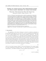
Fig.2. The development of resistivity from 10K to 350K for x =0.03 − 0.07. The inset
shows x =0.00.
For the whole temperature range, both models showed the sharp declines from the
linearity at the temperature near T
N
, whereas the variable hoping model showed relatively
good fit(R
2
> 0.95), both above and below T
N
(Fig.3).
Fig.3. The fits for the small polaron hoping model for two cases x =0.03 and 0.05 (other
two cases are omitted for clarity) show the sharp declines from the linearity at the
temperatures near T
N
. The linear approximation in the high temperature region
has R
2
> 0.98.The inset shows the fit due to the variable hoping model. Although
the linearity was less, this fits the whole temperature range well.
52 Phung Quoc Thanh, Hoa ng Nam Nhat, Bach Thanh Cong
In Fig.4 we show the differential curve dln(ρ)/d(1/T ) drawn together with the
original ln(ρ) vs. 1000/T curve for x =0.03. As seen, the ln(ρ)dropsatthelower
T. Since the dln(ρ)/d(1/T ) corresponds to the activation energy, its drop signifies the

variation of this energy and for our case, this means the change in conduction mechanism.
The estimation for W
P
from the slopes of log (ρ/T ) vs. 1000/T yields 0.52, 0.43, 0.27 and
0.17eV for x =0.00 − 0.07, in sequence.
Fig.4. The differential curve dln(ρ)/d(1/T ) drawn against 1/T for x =0.03 reveals the
drop of the activation energy when the temperature decreases. This argues for the
change in conduction mechanism away from the bandwidth-controlled conduction
to the possible boundary-controlled percolative conduction.
To fit the data in the low temperature region we estimated the fractal dimension
D, needed in relation (7), according to the following procedure. First, measure the total
area of eac h SEM photograph, then divide this area into the smaller squares and use them
to fill each grain area. The number of squares filled into one grain is just the G − area
and the number of squares that cross-over the grain or run over the grain boundary is just
the linear extend G − Length. The log-log plot from these two quantities determines D
(Fig.5).
Fig.5. The log(G − Area)vs.log(G − Length)plot.
Model of conductivity for perovskites based on 53
Table 1 summarizes the m easurement details and results (D, f, L and L

). For the
calculation of f, the percolation threshold concentration x
c
was set to zero since all samples
are above threshold; the concentration x was set equal to the Mn
4+
/M n
3+
ratio estimated
by the Rietveld refinement [9] (also see Rao and Raychaudhury in [5]) a nd D


was assumed
equal to D. A larger grain size L tends to the smaller D.TheseD-s correspond well to
the W
P
, except for x =0.00, as seen in Fig.7.
Fig.6 shows the fit results for two cases x =0.03 and 0.05 (the inset). The dotted
lines denote the fit according to the small polaron model (4) whereas the lines are according
to (7). The least square figure of merit R<0.02. The temperature at which the lines and
the dotted lines cross over is 120K (x =0.03) and 110K (x =0.05). This temperature
drops to 100K for x =0.07. Compared to FC curves [10], these temperatures correspond to
the Neel temperature T
N
of the charge-ordering antiferromagnetic-to-paramagnetic phase
transitions. Table 2 lists the power factor n, the constant ρ
0
and ρ
1
that were determined
from the fits. The n grew linearly with W
P
better than D with W
P
(Fig.7).
Fig.6. The fitexamplesforx =0.03 and 0.05 (the inset) according to (4) (high T region)
and (7) (low T region). The least square figure of merit R<0.02. The cross points
showed the estimated T
N
for each case to be 120K (x =0.03) and 110K (x =0.05).
Recall the approximation for the boundary resistivity was 6 × 10

2
Ωcm [5,7] (con-
firmed to the very low boundary conductivity of 10
−5
in unit of e
2
/W). Our model esti-
mated the pure boundary resistivity to be ρ
0
of order 50 × 10
−5
Ωcm (Table 2), which
suggests the conductivity of order 10 e
2
/W.Sincethe(e
2
/W) corresponds to the minimal
54 Phung Quoc Thanh, Hoa ng Nam Nhat, Bach Thanh Cong
Mott conductivity, the value of 10 is a much better estimation for the boundary conduc-
tivity than the one 10
−5
reported earlier.
Fig.7. The relations between D, n and W
p
show almost linearity between n and W
p
,
whereas this linearity holds for D only if excluding the case x =0.00.
Conclusions
This w ork is the first of its kind to apply the fractal analysis to study the boundary

conduction in pero vskites. The use of the fractal tec hnique in perovskites faces several
limitations due to the small size of the samples that usually do not allow the manufacture
of the Werner array electrode matrix. We showed that by using the SEM images, the
boundary fractal dimension and the related boundary geometric properties, such as the
average size and thickness, might be well estimated, and that the estimated values suc-
cessfully described the temperature behaviours of the resistivity for the tested samples.
Furthermore, the fractal dimension showed very good correspondence to the small polaron
hoping energy in the high temperature region. They also developed linearly with the crit-
ical exponents n in the lo w temperature region; this fact argues for the fractal nature of
n, but the confirmation needs further investigation. In contrast to the fractal dimension
determined on the basis of the voltage drop distribution across the Werner array matrix,
the dimension measured using the SEM images really belongs to the boundary system but
it lacks to bind to the apparent resistivity by its nature. At this stage, their incorporation
into the relation (7) was purely a model. To confirm this model, one needs to arrange the
Model of conductivity for perovskites based on 55
Werner array matrix on the samples, that is to build at least 40 × 40 electrodes onto a
surface area approx. 1cm
2
. We leave this experiment for the future consideration.
References
1. Daolun Chen, Dexing Pang, Zhongjin Yang, Sa Kong, Litian Wang, Ke Yang
and Guiwen Qiao, The relationship bet ween superconductivity and microstructure
through the fractal dimensions in Y-Ba-Cu-O compounds, J. Phys. C: Solid State
Phys. 21(1988), L271-L276.
2. J.C. Phillips, Superconducting and Related Oxides: Ph ysics and Nanoengineering
III, SPIE Proc.,(Ed.D.PavunaandIBozovic),3481(1998) p. 87.
3. J. C. Phillips, Fractal Nature and Scaling Exponents of Non-Drude Currents in
Non-Fermi Liquids, arXiv:cond-mat/0104095.
4. G. Dobrescu, D. Berger, F. Papa, N. I. Ionescu, M. Rusu, Fractal analysis of micro-
graphs and adsorption isotherms of La1-xSrxCoO3 samples, Journal of Optoelec-

tronics and Advanced Materials, Vol.5, No.5(2003).
5. C.N.Rao and B. Raveau, Collossal Magnetoresistance, Charge Ordering and Related
Properties of Manganese Oxides, World Scientific Publishing Co., Singapore 1998.
6. S.S.Krylov, V.F.Lubchich, The Apparent Resistivity Scaling and Fractal Structure
of an Iron Formation, Izvestia, Physics of the Solid Earth,Vol.38No.12(2002), pp.
1006-1012. Translated from Fizika Zemli, No 12, 2002, pp 14-21.
7. A. Gupta, G. Q. Gong, Gang Xiao, P. R. Duncombe, P. Lecoeur, P. Trouilloud,Y.Y.
Wang, V. P. Dravis and J. Z. Sun, Phys.Rev.B54(1996) R15629.
8. B.B . Mandelbrot, The Fractal Geometry of Nature, W.H. Freeman and Co., New
York, NY 1983, (Chapter IV, 12 Length-Area-Volume Relations), p. 110-111.
9. P. Q. Thanh, H.N. Nhat and B.T. Cong, VNU J. of Science, T.XX, No.3 AP, (2004),
p. 130-132.
10. P. Q. Thanh, B.T. Cong, N.N. Dinh, Private communication.