WIRELESS AD-HOC NETWORKS docx
Bạn đang xem bản rút gọn của tài liệu. Xem và tải ngay bản đầy đủ của tài liệu tại đây (6.18 MB, 172 trang )
WIRELESS AD-HOC
NETWORKS
Edited by Hongbo Zhou
Wireless Ad-Hoc Networks
/>Edited by Hongbo Zhou
Contributors
Hongbo Zhou, Takuya Yoshihiro, Paul Muhlethaler, Bartlomiej Blaszczyszyn, Tat Wing Chim, S. M. Yiu, Lucas C. K. Hui,
Victor O. K. Li, Li Liu, Xianyue Li, Jiong Jin, Zigang Huang, Ming Liu, Marimuthu Palaniswami, Shiwen Mao, Yingsong
Huang, Phillip Walsh, Yihan Li, Di Yuan, Vangelis Angelakis, Niki Gazoni
Published by InTech
Janeza Trdine 9, 51000 Rijeka, Croatia
Copyright © 2012 InTech
All chapters are Open Access distributed under the Creative Commons Attribution 3.0 license, which allows users to
download, copy and build upon published articles even for commercial purposes, as long as the author and publisher
are properly credited, which ensures maximum dissemination and a wider impact of our publications. After this work
has been published by InTech, authors have the right to republish it, in whole or part, in any publication of which they
are the author, and to make other personal use of the work. Any republication, referencing or personal use of the
work must explicitly identify the original source.
Notice
Statements and opinions expressed in the chapters are these of the individual contributors and not necessarily those
of the editors or publisher. No responsibility is accepted for the accuracy of information contained in the published
chapters. The publisher assumes no responsibility for any damage or injury to persons or property arising out of the
use of any materials, instructions, methods or ideas contained in the book.
Publishing Process Manager Danijela Duric
Technical Editor InTech DTP team
Cover InTech Design team
First published December, 2012
Printed in Croatia
A free online edition of this book is available at www.intechopen.com
Additional hard copies can be obtained from
Wireless Ad-Hoc Networks, Edited by Hongbo Zhou
p. cm.
ISBN 978-953-51-0896-2
free online editions of InTech
Books and Journals can be found at
www.intechopen.com
Contents
Preface VII
Section 1 MAC Protocols for Wireless Ad-Hoc Networks 1
Chapter 1 Comparison of the Maximal Spatial Throughput of Aloha and
CSMA in Wireless Ad-Hoc Networks 3
B. Blaszczyszyn, P. Mühlethaler and S. Banaouas
Chapter 2 A Distributed Polling Service-Based Medium Access Control
Protocol: Prototyping and Experimental Validation 23
Yingsong Huang, Philip A. Walsh, Shiwen Mao and Yihan Li
Section 2 Routing Protocols for Wireless Ad-Hoc Networks 53
Chapter 3 Graph-Based Routing, Broadcasting and Organizing Algorithms
for Ad-Hoc Networks 55
Li Liu, Xianyue Li, Jiong Jin, Zigang Huang, Ming Liu and Marimuthu
Palaniswami
Chapter 4 Probabilistic Routing in Opportunistic Ad Hoc Networks 75
Vangelis Angelakis, Niki Gazoni and Di Yuan
Chapter 5 Reducing Routing Loops Under Link-State Routing in Wireless
Mesh Networks 101
Takuya Yoshihiro and Masanori Kobayashi
Section 3 Applications of Wireless Ad-Hoc Networks 121
Chapter 6 Review of Autoconfiguration for MANETs 123
Hongbo Zhou and Matt W. Mutka
Chapter 7 Privacy-Preserving Information Gathering Using VANET 145
T. W. Chim, S. M. Yiu, Lucas C. K. Hui and Victor O. K. Li
ContentsVI
Preface
A wireless ad-hoc network is a wireless network deployed without any infrastructure. In
such a network, there is no access point or wireless router to forward messages among the
computing devices. Instead, these devices depend on the ad-hoc mode of their wireless net‐
work interface cards to communicate with each other. If the nodes are within the transmis‐
sion range of the wireless signal, they can send messages to each other directly. Otherwise,
the nodes in between will forward the messages for them. Thus, each node is both an end
system and a router simultaneously.
The wireless ad-hoc network can be divided into several subcategories. With a Mobile Ad-
hoc Network (MANET), the nodes are free to move arbitrarily. Thus, the network topology
keeps changing, and these nodes are constrained by the power supply and computation ca‐
pability. While inFor some other scenarios like such as a wireless mesh network, some nodes
stay fixed. Because these nodes have access to continuous power supply and the Internet,
they have access to relatively less restrained resources. A special case of MANET is Vehicle
Ad-hoc Network (VANET), in which the on-board computer is integrated with a transceiver
and additional accessories and gadgets, which makes the communications between vehicles
or between vehicle and roadside device possible. One feature of the VANET is that the no‐
des (vehicles) move along predefined trajectory (streets and roads). Another feature is that
the lifetime of some wireless links is short-termed.
The wWireless ad-hoc networks has have been gaining its popularity due to several reasons:
(1) there are an abundance of all sorts of mobile devices and sensors that support wireless
connections; (2) without the necessity of infrastructure, it is fast, convenient, and economical
for deployment; (3) it facilitates access to and sharing of digital information anywhere and
anytime without human configuration or maintenance.
There are an array of applications of wireless ad-hoc networks in the place where there is no
infrastructure or the infrastructure is knocked out, and a wireless ad-hoc network is the only
option to share data and information between users. For instance, a temporary wireless net‐
work could be created to connect laptops and other devices during a field trip in a forest/
desert/island, regardless ifno matter the users move around or stay put. With a MANET es‐
tablished among firefighters, police, and paramedics, they could share information to re‐
spond to an emergency more efficiently, which could mean saving a life. A similar scenario
is that in the battlefield, soldiers, tanks, helicopters, and airplanes could use a MANET to
share surveillance data in order to improve the precision and efficiency of attack and chance
of survival. A wireless mesh network can be created among sensor nodes to collect and for‐
ward all sorts of data to a central station. A VANET is an indispensible component in a
smart transportation system. Each car becomes the producer and consumer of traffic infor‐
mation, including but not limited to traffic light status, traffic jam, accidents, road work,
weather, and parking lot vacancy. Other information, like the planned itinerary and the next
turn/lane/exit to pick may also be shared with privacy concerns taken care ofconsidered.
The collection of the data and information will travel along vehicle-to-vehicle links or the
links between vehicles and road-side devices that are connected to the Internet. Eventually
they will be fed into the driverless system to make commuting safer and more relaxing.
Due to the intrinsic characteristics of node instability, limited computation resources, band‐
width, and power supply, constant topology change, distributed operations, and lack of cen‐
tralized management, it is challenging for the design and implementation of network appli‐
cations and protocols for a wireless ad-hoc network. Generally speaking, although the idea
and principles of design and protocols for a hardwired network can be referred to, they can‐
not be ported directly to a wireless ad-hoc network. Their design needs to be adapted or
started from scratch to achieve efficiency or optimization under a new set of constraints.
Dr. Hongbo Zhou
Associate Professor,
Department of Computer Science,
Slippery Rock University, USA
PrefaceVIII
Section 1
MAC Protocols for Wireless Ad-Hoc Networks
Chapter 1
Comparison of the Maximal Spatial Throughput of
Aloha and CSMA in Wireless Ad-Hoc Networks
B. Blaszczyszyn, P. Mühlethaler and S. Banaouas
Additional information is available at the end of the chapter
/>Provisional chapter
Comparison of the Maximal Spatial Throughput of
Aloha and CSMA in Wireless Ad-Hoc Networks
B. Blaszczyszyn, P. Mühlethaler and S. Banaouas
Additional information is available at the end of the chapter
10.5772/53264
1. Introduction
Multiple communication protocols are used to organize transmissions from several sources (network
nodes) in such a way that scheduled transmissions are likely to be successful. Aloha is one of the most
common examples of such a protocol. A major characteristic of Aloha is its great simplicity: the core
concept consists in allowing each source to transmit a packet and back-off for some random time before
the next transmission, independently of other sources. The main idea of the Carrier-Sense Multiple
Access technique (CSMA) is to listen before sending a packet. CSMA is perhaps the most simple and
popular access protocol that integrates some collision avoidance mechanism.
Simple classical models allow one to analyze Aloha and CSMA (see [1, 2]). They show that CSMA
significantly outperforms Aloha as long as the maximum propagation delays between network nodes
remain small compared to the packet transmission delays. However these models are not suitable
for a wireless multihop network context, as they do not take into account the specificity of the
radio propagation of the signal. Consequently, they cannot capture the spatial reuse effect (i.e., the
possibility of simultaneous successful wireless transmissions) which is a fundamental property of
multihop wireless communications.
Intuitively, it could be inferred that the collision avoidance embedded in CSMA should provide a greater
spatial throughput than Aloha’s purely random technique. Despite the large number of studies which
evaluate Aloha and CSMA, to the authors’ best knowledge there is no “fair” comparison of the spatial
throughput of the two schemes in wireless multihop ad-hoc networks
1
. The aim of this paper is to carry
out such a comparison and to quantify the gain in spatial throughput of CSMA over Aloha. We also
study the effect of the various parameters on the performances. To do so, we model the geographic
locations of network nodes by a planar Poisson point process and use the standard power-law path-loss
1
[3] is the only similar study we know of but we explain in this paper why the comparison presented in [3] is not, in our opinion,
“fair” according to us.
©2012 Blaszczyszyn et al., licensee InTech. This is an open access chapter distributed under the terms of the
Creative Commons Attribution License ( which permits unrestricted
use, distribution, and reproduction in any medium, provided the original work is properly cited.
© 2012 Blaszczyszyn et al.; licensee InTech. This is an open access article distributed under the terms of the
Creative Commons Attribution License ( which permits
unrestricted use, distribution, and reproduction in any medium, provided the original work is properly cited.
2 Mobile Ad-Hoc Networks
function of the Euclidean distance to model the mean attenuation of the signal power. Regarding radio
channel conditions, we consider both standard Rayleigh and negligible fading. We use a SINR model
in which each successful transmission requires that the receiver is covered by the transmitter with a
minimum SINR.
For Aloha (both slotted and non-slotted), the above model lends itself to mathematical analysis as shown
in [4, 5]. We adopt use and develop this approach and use simulations (which confirm the analytical
results) to evaluate and optimize the performances of Aloha. The performance of the CSMA in the
previous model is very complex thus we use simulations to study it.
The main contribution of this paper is the analysis and comparison of the performances of slotted,
non-slotted Aloha and CSMA, all optimized to maximize the rate of successful transmissions, under
various radio propagation assumptions (path-loss exponent, fading conditions). Our main findings of
this analysis are:
• CSMA always outperforms slotted Aloha, which in turn outperforms non-slotted Aloha. In a
moderate path-loss scenario (path-loss exponent equal to 4), without fading and the SINR level
required for capture equal to 10, CSMA offers approximately a 2.4 times larger rate of successful
transmissions than slotted Aloha and approximately a 3.2 times larger rate than non-slotted Aloha.
• The advantage of using CSMA is slightly reduced by increasing path-loss decay.
• This advantage is significantly reduced by the existence of fading since CSMA is much more
sensitive to channel randomness than Aloha. In particular, for Rayleigh fading the above comparison
of CSMA to slotted and non-slotted Aloha gives the ratios 1.7 and 2.3, respectively.
• The advantage of using CSMA increases with the SINR capture level.
• The above observations are valid when the transmissions are roughly scheduled to nearest neighbors
and all the three MAC schemes are optimally tuned. This optimal tuning results in scheduling
each node for transmission for about 8%, 6% and 4% of the time, for CSMA, slotted and
non-slotted Aloha, respectively. These values do not depend on the network density, provided the
nearest-neighbor receiver scheduling is used.
• The optimal tuning of CSMA is obtained by fixing the carrier-sensing power level (used to detect if
the channel is idle) to about 8% of the useful signal power received at the nearest neighbor distance.
This makes the transmissions successful with a high probability (from 0.8 to 0.95). Both smaller
and larger values of the carrier-sensing threshold lead to essentially suboptimal performance of
CSMA and sometimes even comparable to that of slotted Aloha. This might explain the apparent
contradiction of our results to those of [3], which indicate similar performance of Aloha and CSMA.
This paper also contributes to the development of the mathematical tools for Aloha by showing that the
so-called spatial contention factor cf [6], appearing in the Laplace-transform characterization of the
interference, is larger in non-slotted Aloha than in slotted Aloha under the same channel assumptions,
by a factor that depends in a simple, explicit way only on the path-loss exponent; cf. Fact 3.2. We also
suggest the usage of the Bromwich contour inversion integral, developed in [7], to evaluate the coverage
probability in the no-fading case; cf. Fact 3.6.
In this paper we will not take into account second order factors such as the back-off strategy in CSMA
or guard intervals in slotted Aloha. We will briefly discuss these factors at the end of the paper to show
that they cannot change the order of magnitude of the comparison between Aloha and CSMA.
The remaining part of this paper is organized as follows. In Section 1.1) we recall some previous
studies of Aloha and CSMA. Section 2 introduces the model: distribution of nodes, channel and capture
assumptions. It also describes in more detail the three MAC protocols studied in this paper. In Section 3
Wireless Ad-Hoc Networks4
Comparison of the Maximal Spatial Throughput of Aloha and CSMA in Wireless Ad-Hoc Networks 3
10.5772/53264
we present our analysis tools. Section 4 provides our findings regarding the performance of the MAC
protocols considered. The conclusions are presented in Section 5.
1.1. Related work
Aloha and Time Division Multiple Access (TDMA) are the oldest multiple access protocol. Aloha,
which is the “mother” of random protocols, was born in the early seventies, the seminal work
describing Aloha [8] being published in 1970. Since that time it has become widespread in various
implementations. The essential simplicity of Aloha also allows for simple analysis. A first, and now
widely taught result regarding the ratio of successful transmissions (cf. e.g [2, 4.2]) was obtained
assuming an aggregate, geometry-less process of transmissions following a temporal Poisson process,
with some overlapping of two or more packet transmissions necessarily leading to a collision. In this
model, the ratio of successful transmissions can reach 1/
(2e) ≈ 18%, when the scheme is optimized
by appropriate tuning of the mean back-off time (intensity of the Poisson process). It was also shown,
that this performance can be multiplied by 2 in slotted-Aloha, when all the nodes are synchronized and
can send packets only at the beginning of some universal time slots.
Although Aloha was primarily designed to manage wireless networks, the lack of a geometric
representation of node locations in the above model makes it unsuitable for wireless networks. To the
authors’ best knowledge, it is in the paper by Nelson and Kleinrock [9] that Aloha was first explicitly
studied in a wireless context. The authors showed that under ideal circumstances with slotted Aloha the
“expected fraction of terminals in the network that are engaged in successful traffic in any slot does not
exceed 21%”. Despite the very simple on-off wireless propagation model used in the paper, this result,
as we will show, is surprisingly close to the results that can be obtained using more recent and more
sophisticated, physical propagation and interference models (cf. [4, 6]) in the case of the fading-less
channel model with the mean path-loss decay equal to 3.5. The key element of this latter approach is
the explicit formula of the Laplace transform of the interference created by a Poisson pattern of nodes
using Aloha. This analysis was recently extended to non-slotted Aloha in [5]. We adopt this approach
and slightly extend it in the present paper.
In the widely referenced paper [10] another simplified propagation model was used to study local
interactions of packet transmissions and the stability of spatial Aloha.
CSMA was studied in the 70s in [1] and in the 90s in articles such as [11]. In these studies, the spatial
reuse is usually not considered. However a few articles such as [12–14] take it into account by modeling
carrier sensing with a graph. Nodes within carrier sense are linked vertices in this graph. However this
model only approximates the carrier-sensing and the capture effect. [15] uses the same model for
CSMA to study the per-flow throughput in the network. Other simplified models of the carrier sensing
and capture effect are proposed in [16, 17].
At the end of the 90s, an original and well referenced study tried to capture the behaviour of the IEEE
802.11 distributed medium access algorithm [18]. Although this study represented a step forward in the
analysis of the IEEE 802.11 collision avoidance mechanism, [18] did not include an accurate model to
capture interference. Thus the spatial throughput of IEEE 802.11 cannot be analyzed with this model.
Although numerous papers are actually using models close to that of [18], they are all unable to compute
the spatial throughput of IEEE 802.11.
In contrast to [18], [19] studies the behaviour of a CSMA network using a more realistic model for
interference and for the capture of packets. However [19] cannot obtain closed formulas and [19] is
actually a semi analytical model based on a Markov chain. Moreover this model can only handle a few
dozen nodes. Thus it cannot easily compute average performance or investigate the effect of the network
parameters. New models have recently appeared such as [20]. These models use the Matern hard core
Comparison of the Maximal Spatial Throughput of Aloha and CSMA in Wireless Ad-Hoc Networks
/>5
4 Mobile Ad-Hoc Networks
process to model the pattern of simultaneously transmitting nodes in a CSMA network. These models,
which allow the spatial throughput to be evalutated, have many flaws. First, CSMA is not accurately
modeled by the Matern hard core process. Secondly the interference is also only approximated. Lastly
the formulas obtained in these models to obtain the throughput are complex and it is difficult to use
them to optimize the protocol when we vary the network parameters. Despite the many papers trying
to analyze the performance of CSMA with spatial reuse, we believe that none of these papers offers
a method for precise and straightforward evaluation of the gain from using the collision avoidance
mechanism of CSMA, in the same framework (infinite Poisson ad-hoc network) in which spatial Aloha
can been analyzed. Thus, for this paper we chose to rely on simulations to estimate the performance of
CSMA. We believe that, for our purpose, this approach offers a faster, more accurate method which is
also easy to implement.
We also want to recall the original geometric approach, also by Nelson and Kleinrock, presented in [3].
Their seminal paper presents a comparison of the performance of Aloha and CSMA in the geometric
setting with the simple on-off wireless propagation model. Such a comparison is also the goal of our
present study which however uses a more realistic propagation and interference model (see above). Our
conclusions appear to differ from those of [3], where the performance of CSMA is found comparable to
Aloha. We show that CSMA, with an appropriately tuned sensing threshold, can essentially outperform
Aloha. The reason for this difference is presumably not due to the different wireless channel models,
but primarily because of a sub-optimal tuning of the CSMA in [3], consisting of too small a sensing
range (taken to be equal to the transmission range). In that sense [3] does not provide a fair comparison
of the spatial throughput of Aloha and CSMA whereas, we believe, our paper does. [21] also compares
Aloha and CSMA but only in terms of outage probability; [21] does not derive the density of successful
transmission.
2. Models
In this section we present the models, which will be used to evaluate and compare the performance of
the CSMA and Aloha MAC schemes.
2.1. Distribution of nodes and channel model
The model that we use here was proposed in [4]; we call it the Poisson Bipole model. It assumes that
the nodes of a Mobile Ad hoc NETwork (MANET) are distributed on the infinite plane according to a
homogeneous, planar Poisson point process of intensity λ nodes per unit surface area (say per square
meter). Each node of this network transmits a packet to its own dedicated receiver located at random
within a distance r meters from it, which is not a part of the Poisson point process. In this paper we
choose r
= a/
√
λ, for some constant a > 0, i.e. of the order of the mean distance to the nearest
neighbor in a Poisson point process of intensity λ. This choice mimics the nearest neighbor scenario.
We also assume that every node has always a pending packet to send. We believe that this assumption
represents the behaviour of a loaded network and allows us to compute the maximum throughput of the
network in a multihop context.
Using the formalism of the theory of point processes, we will say that a snapshot of the MANET
can be represented by an independently marked Poisson point process (P.p.p)
Φ
= {(X
i
, y
i
)}, where
the locations of nodes Φ
= {X
i
} form a homogeneous P.p.p. on the plane, with an intensity of λ,
and where the mark y
i
denotes the location of the receiver for node X
i
. We assume here that one
receiver is associated with only one transmitter and that, given Φ, the vectors
{X
i
− y
i
} are i.i.d with
|X
i
−y
i
| = r.
Wireless Ad-Hoc Networks6
Comparison of the Maximal Spatial Throughput of Aloha and CSMA in Wireless Ad-Hoc Networks 5
10.5772/53264
We assume that whenever node X
i
∈ Φ transmits a packet it emits a unit-power signal that is propagated
and reaches any given location y on the plane with power equal to F/l
(|X
i
−y|).
l
(u)=(Au)
β
for A > 0 and β > 2 (1)
and
|·|denotes the Euclidean distance on the plane. Regarding the distribution of the random variable
F, called for simplicity fading, we will consider two cases:
• constant F
≡ 1, called the no fading case,
• exponential F of parameter 1; this corresponds to the Rayleigh fading in the channel.
2.2. Successful transmission
It is natural to assume that transmitter X
i
successfully transmits a given packet of length B to its receiver
y
i
within the time interval [u, u + B] if
SIR
=
F/l(|X
i
−y
i
|)
¯
I
≥ T , (2)
where T is some signal-to-interference (SIR) threshold and where
¯
I is the average interference suffered
by the receiver y
i
during this packet transmission interval
¯
I
=
1
B
u
+
B
u
I(t) dt , (3)
with
I
(t)=
∑
X
j
∈
Φ,X
j
�=
X
i
F
j,y
i
/l(|X
j
−y
i
|)1I(X
j
transmits at time t) . (4)
Note that taking (2) as the successful transmission condition, we ignore any external noise. This is a
reasonable assumption if the noise is significantly smaller than the interference power
¯
I, which is the
case in our setting.
2.3. MAC protocols
We will assume a saturated traffic model, i.e, that each node always has a packet to transmit to its
receiver. The times at which any given node can transmit are decided by the Medium Access Protocol
(MAC). In this paper we study three MAC protocols: CSMA, slotted Aloha and non-slotted Aloha.
2.3.1. CSMA
The basic rule of CSMA is very simple: each node ready to transmit a packet listens first to the channel
and transmits only if it finds the channel idle. Otherwise it waits for the channel to be idle and further
postpones its transmission attempt for an additional random "back-off" time used to select a single node
among the nodes blocked by the previous transmission. We assume that this random "back-off" time is
Comparison of the Maximal Spatial Throughput of Aloha and CSMA in Wireless Ad-Hoc Networks
/>7
6 Mobile Ad-Hoc Networks
very small and we do not consider it in this study. This assumption is true if the ratio of the propagation
plus detection time over the transmission time of the packet is very small. We discuss at the end of the
article how to introduce corrective terms if propagation and detection times are not negligle.
To decide whether the channel is idle, the sender node computes the interference it receives I
′
. If I
′
≤ θ,
where θ is the carrier-sense threshold then the channel is “idle” otherwise it is busy. The carrier-sense
threshold θ is the main, and in our model, the only parameter that will be tuned to maximize the density
of successful transmissions and thus optimize the performance of the CSMA.
2.3.2. Slotted Aloha
Slotted Aloha supposes that all the network nodes are perfectly synchronized to some time slots (each
of the length B of the packet, common for the whole network) and transmit packets according to the
following rule: each node, at each time slot independently tosses a coin with some bias p which will be
referred to as the Aloha medium access probability (Aloha MAP); it sends the packet in this time slot if
the outcome is heads and does not transmit otherwise.
The Aloha MAP p is the main parameter to be tuned to optimize the access (see a precise description
of the stationary space-time model in [5]).
2.3.3. Non-Slotted Aloha
In non-slotted Aloha all the network nodes independently, without synchronization, send packets (of
the same duration B) and then back off for some exponential random time of mean ε. In a more
formal description of this mechanism one assumes that, given a pattern of network nodes, the temporal
patterns of their retransmission are independent (across the nodes) renewal processes with the generic
inter-arrival time equal to B
+ E where E is exponential (back-off) with mean ε. A precise description of
this stationary space-time model, called the Poisson-renewal model of non-slotted Aloha can be found
in [5]. The analysis of this Poisson-renewal model of Aloha is feasible although it does not lead to
simple closed formulas. In [5] another model, called the Poisson rain model, of non-slotted Aloha has
been proposed. The main difference with respect to the scenario considered above is that the nodes X
i
and their receivers y
i
are not fixed in time. Instead, we may think of these nodes as being “born” at some
time T
i
transmitting a packet during time B and “disappearing” immediately after. The joint space-time
distribution of node locations and transmission instances Ψ
= {(X
i
, T
i
)} is modeled by a homogeneous
Poisson p.p. in 2
+ 1 dimensions with intensity λ
s
= λB/(ε + B). It might be theoretically argued
that the Poisson rain model is a good approximation of the Poisson-renewal model when the density of
nodes λ is large, and the time instances at which a given node retransmits are very sparse. Indeed, the
performance of the Poisson-renewal model is shown in [5] to be very close to that of the Poisson rain
model. Thus, in our analytical study of non-slotted Aloha we will use the results regarding the latter for
simplicity, while in our simulations we use the former.
2.4. Network performance under a given MAC
MAC protocols are supposed to create some space-time patterns of active (transmitting) nodes that
increase the chances of successful transmissions. MAC optimization consists in finding the right
trade-off between the density of active nodes and the probability that the individual transmissions are
successful.
The first step of the analysis of the above trade-off problem consists in evaluating how much a given
MAC protocol contends to the channel; i.e., how many packets it attempts to send per node and per
Wireless Ad-Hoc Networks8
Comparison of the Maximal Spatial Throughput of Aloha and CSMA in Wireless Ad-Hoc Networks 7
10.5772/53264
unit of time. In homogeneous models this can be captured by the average fraction of time a typical
node is authorized to transmit. We will denote this metric by τ. By space-time homogeneity, τλ is the
spatial density of active nodes at any given time and thus τ can also be interpreted as the probability
that a typical node of the MANET is active at a given time. In what follows we will call it thechannel
occupation parameter. The way it depends on the basic (tunable) MAC parameters will be explained
later on.
A complete evaluation of the performance of a MAC protocol must establish the fraction of successful
authorized transmissions. We will denote by p
c
the probability that a typical transmission by a typical
node is successful (given this node was authorized by the MAC to transmit). We call it the cov erage
probability for short. By (2) we have
p
c
= P
0
{F ≥ l(r)T
¯
I }, (5)
where the probability P
0
corresponds to the distribution of the random variables for a typical node
during its typical transmission; this can be formalized using the Palm theory for point processes. This
expression will be the basis of our analytical evaluation of the coverage probability for both slotted and
non-slotted Aloha in Section 3.3. We can notice that
¯
I is independent of F in (5) because our MAC
schemes do not schedule transmissions according to the channel conditions at the receivers.
We define the optimal performance of a given MAC scheme as the situation where the mean number
of successful transmissions per unit of surface and unit of time τλp
c
, called the density of successful
transmissions, is maximized. For a given MANET density λ, this is equivalent to maximizing τp
c
,
which can be interpreted as the probability that a typical node is transmitting at a given time and this
transmission is successful. Following this interpretation, we call τp
c
the mean throughput per node.
It will be analytically evaluated for both Aloha schemes and estimated by simulations for Aloha and
CSMA MAC.
3. Analysis tools
3.1. Simulation scenarios
Our simulations are carried out in a square of 1000 m×1000 m in which we generate a Poisson sample
of MANET nodes with intensity λ
= 0.001 nodes per square meter. For each MANET node we
generate the location of its receiver uniformly on the circle of radius r
= a
√
1000 m centered on this
node. To avoid side effects, we consider a toroidal metric on this square. (Recall that, roughly speaking,
rectangular torus is a rectangle whose opposite sites are “identified”.) Given this metric we consider the
distance dependent path-loss model (1) with some given path-loss exponent β and A
= 1.
Typically β is larger than 2 and smaller than 6. 2 corresponds to free space propagation and 6 is for
situations with a lot of obstacles and reflections. We will use the default value β
= 4; in [22] the
Walfishch-Ikegami model provides β
= 3.8. However in some experiments, we try different values of
β. For each pair of nodes we generate an independent copy of the exponential variable F in the case of
Rayleigh fading or take F
≡ 1 in the no-fading case. Unless explicitly specified, our default value of
the SIR threshold is T
= 10 which is a widely used value.
For a given distribution of nodes we run the dynamic simulation for each of the three MAC schemes
described in Section 2.3 with some particular choice of their main parameters: the carrier-sense
threshold θ for CSMA, MAP p for slotted Aloha and mean back-off time for non-slotted Aloha. The
Comparison of the Maximal Spatial Throughput of Aloha and CSMA in Wireless Ad-Hoc Networks
/>9
8 Mobile Ad-Hoc Networks
packet transmission duration is always B = 1 unit of time. We count both the total number of packet
transmissions and the number of successful transmissions during the simulation, whose total time is
4000 units of time. For CSMA, as already said, we ignore the time spent in back-off when a node, after
having sensed the channel busy, finds the channel idle again before attempting another transmission. In
the simulations we use very small back-off times to select the transmitting nodes and we neglect the time
actually spent in these back-offs. Since each packet transmission takes B
= 1 unit of time, dividing the
number of transmissions by the simulation time and by the number of MANET nodes in the square, we
obtain the one-network-sample estimators of, respectively, the average fraction τ of time a typical node
is authorized to transmit and the mean throughput per node τp
c
. We repeat the above experiment for 10
random choices of the network and take the empirical means of the above one-sample estimators. The
error-bars in all simulation results correspond to a confidence interval of 95%. We use a home-made
event-driven simulator specially dedicated to our simulation problem. This simulatot provides much
faster simulation results than the ones we would obtain with on the shelf simulation tools.
3.2. Analytical results for Aloha MAC
The analytical results for Aloha are based on the (simple) calculation of the average fraction of time
a typical node is authorized to transmit τ and a (more involved) calculation of the Laplace transform
of the interference
¯
I that is the only variable of “unknown” distribution in the expression (5) of the
coverage probability p
c
.
3.2.1. Channel Occupation τ
It is straightforward to see that in slotted Aloha τ
= p. In the Poisson-renewal model of non-slotted
Aloha τ
= B/(B + ε); i.e., the ratio between the packet duration time and the mean inter-transmission
time.
3.2.2. Interference Distribution
The basic observation allowing explicit analysis of the coverage probability for all our Poisson models
of Aloha is that the distribution of the interference
¯
I under the Palm probability P
0
in (5) corresponds
to the distribution of the interference “seen” by an extra receiver added to the original MANET pattern
(say at the origin) during an arbitrary period of time of length B (say in
[0, B]). This is a consequence
of Slivnyak’s theorem.
Moreover, note that in the slotted Aloha MAC the interference I
(t)=I in (3) does not vary during
the packet transmission and consequently
¯
I
= I. Furthermore, note that the pattern of nodes X
j
, which
emit at a given time slot and interfere with a given packet transmission (cf. expression (4)) is a Poisson
p.p. of intensity pλ . This is a consequence of the independent MAC decisions of Aloha. The general
expression of the Laplace transform
L
I
of I, which in this case is a Poisson shot-noise variable, is
known explicitly. Here we recall the expressions for the special cases of interest.
Fact 3.1. For the slotted Aloha model with path-loss function (1) and a general distribution of fading
F with mean 1 we have:
L
I
(ξ)=exp{−λτA
−
2
ξ
2/β
κ}, (6)
where κ
≥ 0 is some constant depending only on the path-loss exponent and the distribution of the
fading F. In particular
Wireless Ad-Hoc Networks10
Comparison of the Maximal Spatial Throughput of Aloha and CSMA in Wireless Ad-Hoc Networks 9
10.5772/53264
• κ = π Γ(1 −2/β) in the no-fading scenario F ≡ 1,
• κ
= 2πΓ(2/β)Γ(1 −2/β)/β with Rayleigh fading.
The constant κ was evaluated in [4] for Rayleigh fading and in [6], for the no-fading scenario, where
the name spatial contention factor was proposed for this constant. Γ
() is the classical gamma function.
Regarding the distribution of the averaged interference
¯
I in non-slotted Aloha, we have the following
new general result.
Fact 3.2. Assume the Poisson rain model of non-slotted Aloha with space-time intensity of packet
transmissions λ
s
= λτ and the path-loss function (1). Assume a general distribution of fading F. Then
the Laplace transform
L
¯
I
(ξ) of the averaged interference
¯
I is given by (6) with the spatial contention
factor κ
= κ
non
−
slotted
equal to
κ
non
−
slotted
=
2β
2 + β
κ
slotted
,
where κ
slotted
is the spatial contention factor evaluated for slotted Aloha under the same channel
assumptions.
Proof. By (3), (4) and exchanging the order of integration and summation we express
¯
I in the following
form
¯
I
=
∑
X
j
∈
Φ,X
j
�=
X
i
F
j,y
i
H
j
/l(|X
j
−y
i
|) ,
where H
j
=
1
B
u
+
B
u
1I(X
j
emits at time t) dt. In the Poisson rain model we have
1I
(X
j
emits at time t)=1I(t − B ≤ T
j
≤ t), where T
j
is the time at which X
j
starts emitting.
Integrating the previous function we obtain H
j
= h(T
j
), where h(s)=(B −|s|)
+
/B and t
+
=
max(0, t). Consequently, for the Poisson rain model represented by Poisson p.p. Ψ = {X
i
, T
i
} (cf.
Section 2.3.3) the averaged interference at the typical transmission receiver is equal in distribution to
¯
I
distr .
=
∑
X
j
,T
j
∈
Ψ
F
j
h(T
j
)/l(|X
j
|) ,
where F
j
are i.i.d. copies of the fading. Using the general expression for the Laplace transform of the
Poisson shot-noise we obtain for the path-loss function (1)
L
¯
I
(ξ)=exp
−2πλ
s
∞
−
∞
∞
0
r
1 −L
F
ξh
(t)(Ar)
−
β
dr dt
,
where
L
F
is the Laplace transform of F. Substituting r := Ar(ξh (t))
−
1/β
for a given fixed t in the
inner integral we factorize the two integrals and obtain
L
¯
I
(ξ)=exp{−2πλ
s
A
−
2
ξ
2/β
ζκ}, where
ζ
=
∞
−
∞
(h(t))
2/β
dt and κ =
∞
0
r(1 −L
F
(r
−
β
)) dr. A direct calculation yields ζ = 2β/(2 + β).
This completes the proof.
Comparison of the Maximal Spatial Throughput of Aloha and CSMA in Wireless Ad-Hoc Networks
/>11
10 Mobile Ad-Hoc Networks
Remark 3.3. Regarding the ratio of the spatial contention parameters ζ = ζ(β)=2β/(2 + β),
that can be seen as the cost of non-synchronization in Aloha (cf Remark 3.5 below), note that in
the free-space propagation model (where β
= 2) it is equal to 1 (which means that the interference
distribution, and so coverage probability, in slotted and non-slotted Aloha are the same). Moreover,
ζ
(β) increases with the path-loss exponent and asymptotically (for β = ∞) approaches the value 2.
This was only conjectured in [5].
3.3. Coverage probability
Evaluating p
c
from (5) is straightforward in the case of Rayleigh fading. Indeed, with F independent of
¯
I one has P
0
{F ≥ l(r)T
¯
I } = E
0
[exp{−l(r)T
¯
I}]=L
¯
I
(l(r)T). By Facts 3.1 and 3.2 we have the
following result.
Fact 3.4. For the Aloha model with the path-loss function (1) and Rayleigh fading
p
c
= exp
−λτr
2
T
2/β
κ
, (7)
where
• κ
= 2πΓ(2/β)Γ(1 −2/β)/β for slotted Aloha and
• κ
= 4πΓ(2/β)Γ(1 −2/β)/(2 + β) for non-slotted Aloha.
Remark 3.5. Note that due to our parametrization r
= a/
√
λ (which mimics the nearest-neighbor
receiver model), the maximal mean throughput per node τp
c
is achieved (in slotted or non-slotted
Aloha with Rayleigh fading) for τ
= τ
∗
= κ
−
1
a
−
2
T
−
2/β
and it is equal to τ
∗
/e. In particular, by
Fact 3.2, non-slotted Aloha achieves ζ
= ζ(β) times smaller maximal throughput than slotted Aloha,
where ζ is the cost of non-synchronization in Aloha. The dependence of this cost on β is analyzed
in Remark 3.3. Here, note only that the well-known result obtained for the simplified collision model
with on-off path-loss function, and saying that slotted Aloha offers two times greater throughput than
non-slotted Aloha (see [2, Section 4.2]) corresponds in our model to the infinite path-loss exponent;
ζ
(∞)=2.
In the case of a general distribution of fading the evaluation of p
c
from the Laplace transform L
¯
I
is not
so straightforward. Some integral formula, based on the Plancherel-Parseval theorem, can be used when
F has a square integrable density. This approach however does not apply to the no-fading case F
≡ 1.
Here we suggest another, numerical approach, based on the Bromwich contour inversion integral and
developed in [7], which is particularly efficient in this case.
Fact 3.6. For Aloha model with constant fading F
≡ 1 we have
p
c
=
2 exp{d/(Tl(r))}
π
∞
0
R
1
−L
¯
I
(d + iu)
d + iu
cos ut du , (8)
where d
> 0 is an arbitrary constant and R (z) denotes the real part of the complex number z.
As suggested in [7], the integral in (8) can be numerically evaluated using the trapezoidal rule and the
Euler summation rule can be used to truncate the infinite series; the authors also explain how to set d in
order to control the approximation error.
Wireless Ad-Hoc Networks12
Comparison of the Maximal Spatial Throughput of Aloha and CSMA in Wireless Ad-Hoc Networks 11
10.5772/53264
3.4. Carrier-sense scaling in CSMA
As mentioned above, a similar analysis of the performance of the CSMA scheme is not possible. If
fact, neither the channel contention described by τ nor the distribution of
¯
I under P
0
is easy to evaluate
for this scheme. Here we want only to comment on some scaling results (with the node density λ)
regarding the performance of CSMA.
Note that in the noiseless scenario (cf SIR condition (2)), with nearest-neighbor-like distance r
=
a/
√
λ from transmitter to receiver, and the path-loss function (1) the SIR is invariant with respect to a
homothetic transformation of the model; i.e., dilating all the distances by some factor, say γ. However,
the received powers (as interference I
′
measured by the transmitters) scale like γ
−
β
. By the well
known scaling property of the homogeneous Poisson p.p.
2
, this implies that the performance of the
CSMA scheme (values of τ and the distribution of
¯
I) in our network model is invariant with respect to
the MANET density provided the carrier-sense threshold θ varies with λ as θ
= θ(λ)=θ(1)λ
β/2
.
In order to present our simulation results for CSMA in a scale-free manner, in Section 4.1 we plot the
mean throughput τ p
c
if the function of the modified carrier-sense threshold is
˜
θ := θl(r) that can be
seen as the power normalized by the received signal power (in contrast to θ that is normalized to the
emitted signal power). This results in
˜
θ
= θ(1)λ
β/2
(Aλ
−
1/2
)
β
= θ(1)A
β
which does not depend on
the density of the MANET.
Another way of presentating scale-free results is to express the carrier-sense threshold θ in terms of the
equivalent carrier-sense distance R defined as the distance at which a unit of emitted power is attenuated
to the value θ, i.e. satisfying θ
= 1/l(R). In our path-loss model this relation makes R = θ
−
1/β
/A.
We will use this approach when comparing our optimal tuning of CSMA to that proposed in [3]; see
Section 4.3.
4. MAC optimization and comparison results
In this section we present our findings regarding analysis and comparison of the performance of Aloha
and CSMA.
4.1. MAC performance study
We study the mean throughput per node τ p
c
achieved by CSMA and Aloha under our default setting
(a
= 1, β = 4, T = 10) with and without fading, depending on the MAC parameters, which are
carrier-sense threshold θ, MAP p and mean back-off time ε for, respectively, CSMA, slotted and
non-slotted Aloha.
4.1.1. CSMA
Figure 1 presents the throughput τp
c
achieved by CSMA versus the modified carrier-sense threshold
˜
θ.
Recall that
˜
θ is the carrier-sense threshold in ratio to the useful power at the received (at the distance
r
= a/
√
λ)
3
. This makes τp
c
and
˜
θ independent of the MANET density; cf. Section 3.4. Our first
observations are as follows.
2
The dilation of a planar Poisson p.p. of intensity 1 by a factor γ
=
λ
−1/2
gives a Poisson p.p. of intensity λ.
3
In other words, e.g.
˜
θ
=
0.1 means that the channel is considered by an emitter as idle if the total power sensed by it is at most
10% of the mean useful signal power received by its receiver.
Comparison of the Maximal Spatial Throughput of Aloha and CSMA in Wireless Ad-Hoc Networks
/>13
12 Mobile Ad-Hoc Networks
Remark 4.1. In the absence of fading the maximum throughput of 0.068 (unit-size packets per unit of
time and per node) is attained by CSMA when the carrier-sense threshold is fixed roughly at the level
of
˜
θ
=
˜
θ
∗
= 0.08. This optimal tuning of the carrier-sense threshold seems to be quite insensitive to
fading. However, the optimal throughput is significantly reduced by fading. Rayleigh fading of mean
1, reduces the CSMA throughput to 63.2% compared with the no fading scenario.
This latter observation is easy to understand as the channel-sensing is done at the emitter and that fading
at the receiver is independent of fading at the emitter.
0.025
0.03
0.035
0.04
0.045
0.05
0.055
0.06
0.065
0.07
0 0.02 0.04 0.06 0.08 0.1 0.12 0.14 0.16 0.18 0.2
τ p
c
Modified carrier-sense threshold
CSMA
Rayleigh fading
no fading
Figure 1. Mean throughput per node τp
c
versus modified carrier-sense threshold
˜
θ in CSMA; Rayleigh fading and no-fading
scenario.
4.1.2. Aloha
Figure 2 presents the throughput τp
c
with and without fading achieved by slotted Aloha versus the
channel occupation time τ, which in this model is equal to the the MAP parameter p. The results of
non-slotted Aloha are presented in Figure 3 with τ
= 1/(1 + ε), where ε is the mean back-off time.
The other parameters are as in the default setting. Here are our observations.
Remark 4.2. In the absence of fading the maximum throughput of 0.028 for the optimal MAP p
=
p
∗
≈ 0.06. As in CSMA, this optimal tuning seems to be quite insensitive to fading, which in the case
of Rayleigh fading can be evaluated explicitly as p
= p
∗
= κ
−
1
T
−
2/ β
(which gives p
∗
= 0.064081
in the default Rayleigh scenario). In contrast to CSMA, Rayleigh fading has a relatively small impact
on the slotted Aloha throughput reducing it only to 92% of the throughput achieved in the no-fading
scenario (in contrast to 63.2% in CSMA). Similar observations hold for non-slotted Aloha, which in the
Rayleigh fading scenario achieves ζ
= 2β/(2 + β)=1.5 times smaller throughput than the slotted
version.
4.2. Impact of model parameters
In Figures 4, 5, 6, 7, 8 and 9 we can study the dependence of the maximal throughput achievable
by the MAC schemes (at their respective optimal tunings) as a function of the path-loss exponent β,
Wireless Ad-Hoc Networks14
Comparison of the Maximal Spatial Throughput of Aloha and CSMA in Wireless Ad-Hoc Networks 13
10.5772/53264
0
0.005
0.01
0.015
0.02
0.025
0 0.05 0.1 0.15 0.2
τ p
c
τ
Slotted Aloha
Rayleigh fading - simulation
Rayleigh fading - model
no fading - simulation
no fading - model
Figure 2. Mean throughput per node τ p
c
versus channel occupation τ
=
p in slotted Aloha; Rayleigh fading and no fading
scenario.
0
0.005
0.01
0.015
0.02
0 0.05 0.1 0.15 0.2
τ p
c
τ
Non slotted Aloha
Rayleigh fading - simulation
Rayleigh fading - model
no fading - simulation
no fading - model
Figure 3. Mean throughput per node τp
c
versus channel occupation time τ
=
1/
(
1
+
ǫ
)
for non-slotted Aloha; Rayleigh
fading and no fading scenario.
SIR threshold T and relative distance to the receiver a (recall that a = r
√
λ). It is clear that CSMA
significantly outperforms both Aloha protocols for all choices of parameters.
More detailed observations are as follows.
Remark 4.3. The higher path-loss exponent β is, the less advantage there is in using CSMA. When
there is no fading, the increase of β from 3 to 6 reduces the gain in throughput of CSMA with respect
to slotted Aloha from 2.6 to 2.1 and with respect to non-slotted Aloha from 3.5 to 3.2.
Comparison of the Maximal Spatial Throughput of Aloha and CSMA in Wireless Ad-Hoc Networks
/>15
14 Mobile Ad-Hoc Networks
0.01
0.02
0.03
0.04
0.05
0.06
0.07
0.08
0.09
0.1
0.11
3 3.5 4 4.5 5 5.5 6
τ p
c
Path loss exponent β
No fading
slotted Aloha
non-slotted Aloha
CSMA
Figure 4. Maximal achievable mean throughput per node τp
c
versus path-loss exponent β in the absence of fading.
0
0.01
0.02
0.03
0.04
0.05
0.06
0.07
0.08
3 3.5 4 4.5 5 5.5 6
τ p
c
Path loss exponent β
Rayleigh fading
slotted Aloha
non-slotted Aloha
CSMA
Figure 5. Maximal achievable mean throughput per node τp
c
versus path-loss exponent β with Rayleigh fading.
We can also see in Figure 4, that in the absence of fading, slotted Aloha attains the expected fraction of
21% of terminals engaged in successful traffic, foreseen in the seminal paper [9], for SINR threshold
T
= 10 and a moderate path loss exponent slightly larger than β = 3.5.
Remark 4.4. The existence of fading (see Figure 5) further diminishes the advantage of CSMA. In
particular, Rayleigh fading reduces the gain in throughput of CSMA with respect to slotted Aloha to
about 1.7 and for non-slotted Aloha to a factor between 2.5 and 2.1 (depending on β).
Studying the impact of the SINR threshold T we observe the following, see Figures 6 and 7.
Remark 4.5. The higher T is (and hence the smaller bit-error rate sustainable in each packet), the
greater is the advantage of using CSMA. In particular, when there is no fading and for β
= 4, increasing
Wireless Ad-Hoc Networks16
Comparison of the Maximal Spatial Throughput of Aloha and CSMA in Wireless Ad-Hoc Networks 15
10.5772/53264
0
0.02
0.04
0.06
0.08
0.1
0.12
0.14
0.16
0 2 4 6 8 10 12 14 16
τ p
c
Capture threshold T
No fading
slotted Aloha
non-slotted Aloha
CSMA
Figure 6. Maximal achievable mean throughput per node τp
c
versus SIR threshold T in the absence of fading.
0
0.02
0.04
0.06
0.08
0.1
0.12
0 2 4 6 8 10 12 14 16
τ p
c
Capture threshold T
Rayleigh fading
slotted Aloha
non-slotted Aloha
CSMA
Figure 7. Maximal achievable mean throughput per node τp
c
versus SIR threshold T. Rayleigh fading.
T from 1 to 11 results in the increase in the gain in throughput of CSMA with respect to slotted Aloha
from 2.4 to 3.5 and this latter ratio remains stable for T larger than 11. For a similar comparison of
CSMA to non-slotted Aloha the gains are from 1.8 to 2.6. In the case of Rayleigh fading the analogous
gain factors of CSMA are, respectively, from 1.8 to 2.4 with respect to slotted Aloha and from 1.4 to
1.8 with respect to non-slotted Aloha.
Finally we study the impact of the relative distance to the receiver a (in ratio to the mean distance to
the nearest neighbor in the network). Figures 8, and 9 show clearly that this distance should be kept as
small as possible without disconnecting the network.
Comparison of the Maximal Spatial Throughput of Aloha and CSMA in Wireless Ad-Hoc Networks
/>17