A Critical Point Anomaly In Saturation Curves Of Reduced Temperat
Bạn đang xem bản rút gọn của tài liệu. Xem và tải ngay bản đầy đủ của tài liệu tại đây (2.01 MB, 16 trang )
The Space Congress® Proceedings
1971 (8th) Vol. 1 Technology Today And
Tomorrow
Apr 1st, 8:00 AM
A Critical Point Anomaly In Saturation Curves Of Reduced
Temperatures -Compressibility Planes Of Pure Substances
Joseph W. Bursik
Associate Professor of Aeronautical Engineering and Astronautics, Rensselaer Polytechnic Institute
Follow this and additional works at: />
Scholarly Commons Citation
Bursik, Joseph W., "A Critical Point Anomaly In Saturation Curves Of Reduced Temperatures
-Compressibility Planes Of Pure Substances" (1971). The Space Congress® Proceedings. 5.
/>
This Event is brought to you for free and open access by
the Conferences at Scholarly Commons. It has been
accepted for inclusion in The Space Congress®
Proceedings by an authorized administrator of Scholarly
Commons. For more information, please contact
A CRITICAL POINT ANOMALY IN
SATURATION CURVES OF REDUCED TEMPERATURE COMPRESSIBILITY PLANES OF PURE SUBSTANCES
Joseph W. Bursik
Associate Professor of
Aeronautical Engineering and Astronautics
Rensselaer Polytechnic Institute
Troy, New York
ABSTRACT
in luring away adherents of the classical view,
Lines of striction are obtained in 9, x, Tr and
Z, x, Tr spaces of one component, two-phase re
gions; 9 being the reduced pressure volume prod
uct, pr vr ; Z, pr vr/Tr and x the quality. Us
ing the concept of smoothly joined saturation
curves at the critical points of Tr , 9 and Tr , Z
planes and a transformation of the striction
curves into the 9, Z plane results in an impos
sible anomaly at the critical point. Removal of
the anomaly necessitates abondoning the concept
of smooth, saturation curves at the critical
points of all of these planes.
In this paper a new, analytical approach is used to
revive the concept of a critical point at which the
saturation curves are joined non- smoothly . This
method uses the combined disciplines of metric dif
ferential geometry and thermodynamics. It utilizes
as its chief tool the geometric concept of the line
of striction associated with the representation of
various thermodynamic functions as ruled, non- de
velopable surfaces. These functions are the re
duced compressibility factor and the reduced pres
sure-specific volume product.
Extended Geometrical Surfaces
INTRODUCTION
In the classical thermodynamics conception of the
critical point terminating the liquid-vapor re
gion of an arbitrary pure substance the coexis
tence curves are always smoothly joined when the
properties are viewed in appropriate planes. In
the pressure - specific volume plane a horizontal
line through the critical point serves as the
tangent line to both the saturated liquid and va
por curves. A similar statement can be made with
regard to the joining of the coexistence curves
at the critical point of any plane in which pres
sure or temperature is plotted as the ordinate
and any function such as the compressibility or
the specific value of entropy, internal energy,
enthalpy, volume, etc., is plotted as the abscis
sa. Indeed, when any two functions from this lat
ter group are cross plotted - as for example in
the Mollier plane - the smoothness concept at the
critical point is still retained. However, the
common critical tangent to the saturated liquid
and vapor curves is no longer a horizontal line
in these planes.
In spite of the general acceptance of this con
cept of critical point smoothness; other views
have appeared in the literature from time to time.
These range from a critical temperature line con
cept ^ to a non-smooth point concept. Mayer and
Harrison,(2,3) for example, envisioned a rather
narrow spike of two-phase region added in the
vicinity of the critical point to the normal twophase region of the p, v plane; and CallenderW
reported strong discontinuities in the saturation
curve slopes at the critical point. However,
these departures from the classical thermodynam
ics smoothness concept have not been successful
4-1
In the liquid-vapor regions of pure substances the
mixture specific volume can be written explicitly
as a function of the quality and implicitly as a
function of the temperature through the dependence
of the saturated liquid and vapor volumes on the
temperature. Thus,
v(x,T) = V
(1)
This enables the compressibility factor and the
pressure-specific volume product, denoted by 9, to
be written for the two-phase region as
Z - (p/RT) (V]L + x v 12)
(2)
+ x
(3)
Introduction of reduced variables transforms these
to
(4)
and
(5)
Finally, Z, Z
iables
and 0, 9
are absorbed into new var
(6)
and
9 - I/I
(7)
such that Equations 4 and 5 become
x V12r>
THE LINE OF STRICTION
(8)
and
(9)
The saturated vapor and saturated liquid values of
these functions are respectively
(10)
(11)
Fr V 2r
and
(p r /T r')v,
vt
JLr*,
(12)
P v rl,
*r
(13)
From these and the fact that the pressure is a func
tion of the temperature, the isothermal phase change
values are formed as
Z 12 = (pr/Tr)v!2r
(14)
For the case of interest of this paper, y-^ will
vary with the temperature; thus, the extended geo
metric surface given by Equation 18 is a non-devel
opable, ruled surface. As such, it has the proper
ty that as the contact point of the surface normal
moves on a ruling from minus infinity to plus in
finity the normal simultaneously rotates about the
ruling through an angle oftf with the rotation being
continuous and in one direction only. This means
that at some intermediate contact point of the same
ruling the surface normal must be turned through an
angle ofTT/g relative to its orientation at either
infinity of the ruling. This intermediate contact
point is called the central point of the ruling.
Thus each ruling has a central point and the locus
of the central points is defined as the line of
striction. This curve which spans the entire tem
perature interval of the two-phase region because
the rulings of the surface of Equation 18 are the
isotherms is of fundamental importance to two-phase
thermodynamics. It will be derived from the proper
ties of the surface normal already described.
The total differential of y is obtained from Equa
tion 18 as
dy =
and
Pr V12r
(15)
When these are substituted into Equations 8 and 9
the results are
l:m:n
(16)
(17)
0:4-1:0.
These two equations have the same form and from a
geometrical point of view they will be treated when
ever possible as one equation of the form
y(x,Tr)
(20)
!2 : yl
When the quality approaches plus or minus infinity
on an isotherm not the critical, the above relation
becomes
and
12
(19)
From this, the direction cosine ratios for the sur
face normal are read as
(18)
That is, if y is replaced everywhere in Equation 18
by Z, Equation 16 results; similarly, substitution
of 0 for y in Equation 18 gives Equation 17.
(21)
That is, the surface normals at the two infinities
of the isothermal ruling are parallel and anti-par
allel to the Tr axis. This means that the surface
normal is rotated 180° at the second infinity rela
tive to the first.
To obtain an expression for the contact point cor
responding to the central point it is only neces
sary to set
Equation 18 represents a ruled surface in y, x, T
space with the reduced isotherms being the rulings,
and x being the quality. When yj^ *- 8 not a constant
the surface is non-developable. Ordinarily the qual
ity is restricted to the physical interval between
zero and one, in effect restricting the rulings to
a finite extent. However, an extended geometric
surface is obtainable from Equation 18 by merely per
mitting the quality to take on values from minus in
finity to plus infinity. In this way the rulings
of the usual thermodynamic surface are extended to
infinite length and the ordinary thermodynamic sur
face becomes a sub-surface of the extended geomet
rical surface.
(22)
Xey y!2
at the central point whose quality is now denoted
by xey . With this, the direction cosine relation
at the central point is obtained from Equations 22
and 20 as
ey
"12
- 1.
As previously mentioned the locus of the central
4-2
(23)
Comparison with Equation 21 shows that the surface
normal at the central point of the ruling is orient
ed at an angle of 90° from the normals at the two
infinities of the same ruling.
points is the line of striction, a space curve whose
x, Tr trace is given by Equation 22. Since y^ and
y12 are temperature functions, it is expected in
general that Equation 22 defines xe as a function
of temperature except in a possible special case
where y{(Tr> is proportional to y{ 2 (Tr). If this
case were possible, then x would be a constant
and the surface becomes a conoid or even a right
helicoid - surfaces that are well understood in met
ric differential geometry. With Equations 18 and
22 the formal description of the line of striction
becomes
(24)
['<•
(Tr)
(25)
(26)
Critical Point Terminal Values of the Striction
Qualities
When the thermodynamic surface is referred to its
line of striction by eliminating y\ in Equation 19
with the substitution of Equation 22 the total dif
ferential of y becomes
dT
y!2 dx '
of the data for all three substances; therefore,
the line of striction quality is always in the phys
ical range of zero to one for all three substances,
as is illustrated for the case of Nitrogen as plot
ted in Figure 2. This is not the case for the re
duced pressure-specific volume product of Nitrogen
where the data shows that 0£ and 0£ are of opposite
sign for reduced temperatures greater than 0.793
but are of the same sign for reduced temperatures
less than 0.793. In the upper temperature interval
the striction curve quality will again be in the
physical range of zero to one; however, for reduced
temperatures less than 0.793 the striction curve
quality is restricted to negative values since both
01 and Q^ are positive, resulting in negative x
when referred to Equation 25 with y used for 0. fl
This is illustrated for Nitrogen in Figure 3, Sim
ilar statements can be made about the data for Oxy
gen and Argon.
(27)
From this, it is apparent that the partial deriva
tive Oy/dT ) is linear in the quality, and when
it is applied to points on an isotherm it vanishes
at the central point. Thus at the central point
viewed in the y, x plane Equation 27 requires that
both the curve of constant temperature and the line
of striction have the same slope. That is, the
line of striction appears as the envelope of the
isotherms in this plane. It is because of this en
veloping property that the central point quality is
given the subscript e. If the surface should be
the conoid or right helicoid previously alluded to,
the envelope degenerates into a point in this plane
which is the. common point of intersection of the
straight line family of isotherms. The degree to
which experimental data in an isolated case approxi
mate this intriguing possibility is shown in Figure
1 whe£e the isotherms are plotted in an "s, x plane.
Here li is the ratio of the entropy to that of sat
urated vapor at the triple point. The substance is
Argon and its two-phase, liquid-vapor^data were ob
tained from Dini°) The equation for "s is quite ob
viously of the form given by Equation 18 if T in
that equation is interpreted as the ratio of the
temperature to the triple point temperature.
Further analysis of the partial derivative
Oy/dTr) x shows that when y' and y' are of oppoposite sign, the central point quality is within
the physical interval and when yl and y" are of
the same sign the line of striction is outside the
physical domain of qualities; that is, negative or
greater than one.
In this paper only two choices for the y function
are studied, namely 0 and Z. In Tables 1, 2 and 3
the saturation values for these two functions are
shown for Nitrogen, ^ Oxygen^ and Argon. ( 6) To
illustrate the preceding discussion Z{ and Z^ are of
opposite sign throughout the temperature interval
4-3
Since y is restricted to represent 0 and Z for the
above substances the Tr , y plane will always have
an upper sub-range of temperatures for the liquidvapor region characterized by yj and y' being of
opposite sign. This means that the qualities asso
ciated with the line of striction in this tempera
ture sub-range which includes the critical are in
the physical range of qualities. The critical point
is the classical one characterized by y * ( 1)—^ 4- o» ,
y£(l)-*-oo and y| 2 <l)-*> -eO .
Because of these infinities at the critical point
the terminal value of the striction curve quality denoted by E - must be obtained at the critical
point by a limiting procedure. That, is, Equation
22 applied to the critical temperature where T . - 1
yields
- 0
E
(28)
However, with both y!(l) and y' (1) being infinite,
the equation obviously will not' yield E . ' Instead
a limiting procedure involving Equation 25 is used
to obtain E as
Ey
li.
yl (Tr>
(29)
This has the disadvantage that the saturation prop
erties of Tables 1, 2 and 3 do not contain the deri
vative data necessary for the evaluation of the
right side of Equation 29; therefore, the deriva
tives must be obtained from, the function tabulations*
This is difficult to do because of the extremely
rapid variation of the properties in.the Immediate
vicinity of the critical point. A method of tangents
is available for estimating all of the x
includ
ing E by plotting yj_ against y^* The slope at
each point of this plot corresponds to minus x *
Finally, the limiting value of the right side of
Equation 29 can be obtained indirectly without re
sorting to derivative analysis. This is accomplish
ed by passing a y = constant curve through the crit
ical point of the T , y plane. Using Equation 18
for this curve and, solving for x leads to .an inde-
terminate form at the critical point. When both
the numerator and denominator of this expression
for x are differentiated with respect to tempera
ture the limit is identical with the right side of
Equation 29. Thus, the terminal quality of the
Z =» Z curve is the same as EZ and the terminal
quality of the 0 - 0Q curve is the same as EQ . For
each substance the pair of numbers E« and Eg - each
between zero and one - can then be obtained graphic
ally by extrapolating the x, Tr plots of the Z = Z c
and 0 = 0C curves to Tr = 1. Actually, it is suf
ficient for the purposes of this paper to know that
the right side of Equation 29 converges to a number
between zero and one. The pair of numbers Eg and
£„ will play a fundamental role in the transforma
tion to the 0, Z plane where the crucial anomaly
will be shown.
because in the region of interest it has been shown
that x fl is a positive number between zero and one.
except at the critical point where
Thus xefl ^ x
Z.J2 is e infinfte, forcing the right side of Equation
37 to be zero at that point, giving the important
result that
U0
Ee - Ez = Eez
Distinctness of the Striction Curves
Before transforming to the 0, Z plane it will first
be shown that the two striction curves implied in
Equation 22, namely e0 and eZ, are distinct except
that they intersect at the critical temperature.
The two curves are made explicit by letting y first
represent 0 and then Z, thus giving
TRANSFORMATION TO THE 0, Z PLANE
and
XeZ Z>12
(31)
d0
dZ
From Equations 12 and 13
1= Z l Tr
(32)
d0
dZl x=k
(33)
12
(34)
and the corresponding derivative
= Tr Z i2
12
(35)
When 0' and 0* are eliminated from Equation 30 by
use of Equations 33 and 35 the result is
VZ i
Xe9Z 12
(36)
Finally Zl is eliminated by use of Equation 31 to
give
eZ
e0
Z i2
(40)
- xeZ )Z i2
(41)
From the latter it follows that at the point of in
tersection of the curve of constant quality with the
e0 striction curve at any temperature but the crit
ical, the slope of the x = k curve is zero. Simi
larly, when the constant quality curve intersects
the eZ striction curve at any temperature other than
the critical, the slope of the constant quality
curve is infinite at the point of intersection.
This requires the e0 curve to appear in the 0, Z
plane as the locus of the zero slope points of curves
of constant quality, and the eZ curve as the locus
of the infinite slope points of these constant qual
ity curves. This is illustrated for Nitrogen, Oxy
gen and Argon in Figures 4, 5 and 6, where these
loci are approximately located on a few x = k curves
for all of these substances.
Similarly Equations 14 and 15 yield
Z l Tr
k 9 12
and
Differentiation gives
ei • Vi
(39)
With this established, attention is now turned to
the interplay of the striction curves and constant
quality curves in the 0, Z plane. From Equations
19 and 27, with y alternately representing 0 and Z,
two different forms are obtained for the slope of a
curve of constant quality, x = k, in the 0, Z plane
as
(30)
e9
(38)
This equation is independent of substance. It de
pends only on the concept of a smoothly rounded sat
uration dome in the vicinity of the critical point
of the T , y plane - where y again alternately rep
resents § and Z. To emphasize the fact that the two
striction curves share a common quality at the crit
ical temperature an additional symbol is defined for
the common quality as EQ_ such that
As previously discussed, these figures also illus
trate that the e0 line of striction for each of these
three substances lies on the physical portion of the
appropriate y, x, Tr space from its terminus at the
critical isotherm to the intersection with the x = 1
curve where 02 has its extremum value. While the
eZ line of striction of these three substances is
entirely within the physical portion of the extended
Z, x^Tr space for the entire temperature range of
the two-phase region, only that portion in the neigh
borhood of the critical point is illustrated.
(37)
From this it is seen that if the two curves defined
by Equations 30 and 31 are identically one curve
at all temperatures, the right
such that XCQ » x
side of the last equation would have to vanish.
and this cannot be
= - ZZ
This means that X
4-4
Up to this point the interplay of these curves has
been studied for points other than the critical.
The approach to the critical point of either of the
two striction curves in terms of intersections with
constant quality curves is not readily discernible;
however, it is susceptible to analysis with the use
of Equation 40. First the 9 terms are eliminated
by use of Equations 33 and 35 to give
d9
dZ
1
x==k
Z1 + k Z
|
|Z .
"i'^"in
1
12
= T +
•"•
By use of Equation 39 these critical point slopes
become
d9
dZ
d9
dZ
(42)
x=E n
Zi
Quite obviously the Efl curve of constant quality
cannot have this double set of critical point slopes.
Indeed, if it were possible, it would mean that an
isotherm in the vicinity of the critical is inter
sected in two distinct points by the same curve of
constant quality and this cannot be.
(43)
As the temperature approaches the critical on this
curve of constant quality the denominator on the
right side of Equation 43 becomes zero by virtue of
Equation 28, with y playing the role of Z; therefore
the slope of the x = E curve becomes infinite at
the critical point. Tnus all x = k curves have an
infinite slope at their points of intersection with
the eZ striction curve.
In view of this result, a recapitulation of the key
points in the chain of argument is offered. The
striction curve relations given by Equations 22, 30
and 31 are, of course, the new ingredients super
posed on the ordinary equations of two-phase thermo
dynamics. The most important striction curve equa
tion in the development is Equation 28 which is the
limiting form at the critical temperature. In Equa
tion 43 and 45 thermodynamics is explicitly blended
with differential geometry such that the applica
tion of Equation 28 to these equations results in
Equations 46 and 47. There is nothing special about these last two equations as long as EQ and E
are thought of as two different curves of constant
quality. Indeed, they represent a continuity prin
ciple in the statement that the distribution of
x = k curve slopes at all points of intersection
with the e9 striction curve is always zero, and
that the distribution of x = k slopes at points of
intersection with the E striction curve is always
infinite. However, when Equation 37 is applied to
the critical temperature assuming Zl« to be infinite
the crucial Equations 38 and 39 result.
When ZJ and z!« are eliminated from Equation 40 by
Equations 33 and 35 the result is
d9
dZ
.
x=k
^ _
Z- + k Z 10
1_____12
(44)
For the constant quality curve x = k « E^ Equation
44 becomes
dZ
x=E_
"
.
Z l + Vl2
L " r\ I
i
(45)
i? ftt
It would appear that the only way to break the
chain of argument is to abandon the assumption that
Z! 7 is infinite at the critical temperature. Then
Equations 38 and 39 will not result from the appli
cation of Equation 37 to the critical temperature.
Then Equations 46 and 47 still exist; however, Equa
tions 48 and 49 do not.
As the critical temperature is approached on this
curve of constant quality the term on the right side
of Equation 45 that involves the saturation 9 is
zero by virtue of Equation 28, with y playing the
role of 9; therefore, the slope of this x = E^
curve is zero at the critical point. Thus all of
the constant quality curves intersected by the e9
striction curve have zero slopes at the intersec
tions as viewed in the 9, Z plane.
The use of a finite, critical Z' in Equation 35
means that the critical value of 9^ 2 is likewise
finite. With both 0' and Z' finite at the criti
cal point then 9', 9*7 Z' ani Z* must also be finite
at this point, and tfie classical concept of a smooth
saturation curve in the vicinity of the critical
point in both the Tr , 9 and Tr , Z planes has to be
abandoned.
In summary, at the critical temperature
d9
dZ
—>> oO
x=Ez
Tr-l
(46)
d9
dZ
= 0.
(47)
Adoption of this view that the critical point values
of the striction curve qualities are finite and un
equal leads to simple expressions in terms of E_
and EO for the critical slopes of the saturation
curves in the various planes. When Equation 37 is
and
x=E
(49)
XFE,
CONCLUSION AND DISCUSSION
L
EZ Z 12
'ez
(48)
Tr-l
Then the curve of constant quality is selected as
x = k = E_ and this converts the last equation to
d9
dZ
x=E,'ez
Tr-l
4-5
APPENDIX
solved for Z| 2 , *-ts critical value becomes
Saturation Values of 0 and Z for Nitrogen
This, together with Equation 35 and Z., 2
9'
*12c =
Table 1
(50)
Z 12c
___1
- E^
= 0, gives
(51)
Coupling these last two equations to Equations 30
and 31 results in
(52)
and
(53)
Tr
el
92
Zl
Z2
0.5005
0.5284
0.5724
0.6132
0.6165
0.6605
0.7045
0.7486
0.7926
0.8366
0.8807
0.9247
0.9687
0.9952
1.0000
0.0013
0.0025
0.0059
0.0115
0.0122
0.0229
0.0399
0.0658
0.1036
0.1576
0.2344
0.3457
0.5226
0.7181
1.0000
1.714
1.798
1.924
2.024
2.033
2.122
2.189
2.230
2.240
2.211
2.135
1.991
1.729
1.424
1.000
0.0027
0.0047
0.0102
0.0188
0.0198
0.0347
0.0566
0.0879
0.1307
0.1884
0.2662
0.3739
0.5395
0.7216
1.0000
3.425
3.402
3.362
3.300
3.297
3.213
3.107
2.979
2.826
2.642
2.424
2.153
1.785
1.431
1.000
From these last four equations and the fact that
y!2 = y2 " yl iC follows that
Table 2
Saturation Values of 0 and Z for Oxygen
(54)
Tr
01
e2
Zl
Z2
0.4826
0.5236
0.5600
0.5828
0.6024
0.6704
0.7120
0.7337
0.8103
0.8625
0.9032
0.9369
0.9659
1.0000
0.0009
0.0024
0.0048
0.0072
0.0099
0.0261
0.0433
0.0552
0.1197
0.1926
0.2752
0.3710
0.4884
1.0000
1.558
1.678
1.778
1.834
1.880
2.011
2.066
2.086
2.099
2.045
1.952
1.825
1.654
1.000
0.0019
0.0045
0.0086
0.0123
0.0165
0.0390
0.0608
0.0753
0.1477
0.2233
0.3047
0.3960
0.5056
1.000
3.228
3.205
3.175
3.147
3.121
3.000
2.902
2.843
2.590
2.371
2.161
1.948
1.712
1.000
and
(55)
Finally, these results are used in the transforma
tion to the 0, Z plane to give
d0
dZ
eic
Ic
Ee
= _i£ = JS
EZ
Z ic
(56)
and
d0
dZ
(57)
Table 3
Saturation Values of 0 and Z for Argon
Multiplication of the right sides of Equations
50, 52 and 54 by Z/I gives the critical point val
ues of dzL 2 /dT, dZ-/§T and dZ2 /dT where Z is the
usual compressibility factor and T is the ordinary
dimensional temperature. Similarly, multiplying
the right sides of Equations 51, 53 and 55 by
*5C/T C gives the critical point values of d^2 /dT,
dB^/dl and
* and d52 /dZ2 are obtained by
cal values of d9
multiplying the righ t sides of Equations 56 and 57
by V z
4-6
Tr
91
e2
Zl
Z2
0.5559
0.5792
0.6266
0.6582
0.7031
0.7363
0.7750
0.8242
0.8627
0.8948
0.9226
0.9695
1.0000
0.0053
0.0079
0.0164
0.0251
0.0434
0.0626
0.0925
0.1467
0.2061
0.2743
0.3516
0.5396
1.0000
1.874
1.939
2.058
2.122
2.186
2.218
2.223
2.200
2.126
2.041
1.985
1.724
1.000
0.0095
0.0137
0.0262
0.0381
0.0617
0.0851
0.1194
0.1780
0.2389
0.3065
0.3811
0.5566
1.0000
3.370
3.348
3.328
3.224
3.109
3.012
2.868
2.669
2.464
2.281
2.152
1.778
1.000
NOMENCLATURE
E
ILLUSTRATIONS
- terminal (critical temperature) value of the
line of striction quality of y(x, T ) space,
dimensionless.
r
p
- absolute pressure pounds per square foot.
R
- specific gas constant, foot pounds per pound
_
mass deg R
s
- specific entropy divided by triple point sat
uration specific entropy, dimensionless.
^T
- absolute temperature, degrees Rankine.
9
- pressure-specific volume product, foot pounds
per pound_mass.
9
- ratio 6/0 c , dimensionless
v
- specific volume, cubic feet per pound mass
x
- quality, dimensionless
xey - quality on the line of striction of y(x, Tr)
space, dimensionless
y
- generalized thermodynamic property; alternate_
ly used for 9 and Z, dimensionless
Z
- compressibility factor, pv/RT, dimensionless
Z
- ratio Z/Z C , dimensionless
Prime - differentiation of any temperature function
with respect to temperature
y
Subscripts
c
r
1
2
12
- critical point value.
- reduced property; ratio of actual property
value to critical point value.
- saturated liquid
- saturated vapor
- isothermal difference, saturated vapor value
minus saturated liquid value.
REFERENCES
(1) Rice, O.K., J. Chem. Phys. 15, 314; errata,
615 (1947.
(2) Mayer, J.E. and Harrison, S.F., J. Chem. Phys.
6, 87 (1938).
(3) Harrison, S.F. and Mayer, J.E., J. Chem. Phys.
6, 101 (1938).
(4) Callender, H.L., Proc. Roy. Soc., 120 A, 460
(1928).
(5) Lane, E.P., "Metric Differential Geometry of
Curves and Surfaces", The University of Chicago
Press, Chicago, 111., pp. 92-101,
(6) Din, F., "Thermodynamic Functions of Gases",
vol. 2, Butterworths Scientific Publications,
London 1956.
(7) Van Wylen, G.J. and Sonntag, R.E., "Fundamentals
of Classical Thermodynamics," John Wiley and Sons,
N.Y. (1965).
4-7
FIGURE CAPTIONS
FIGURE 1.
Isothermals in the Is, x Plane of Argon.
FIGURE 2.
Striction Curve and Constant Quality
Curves in the Tr> Z Plane of Nitrogen.
FIGURE 3.
Striction Curve and Constant Quality
Curves in the Tr , 6 Plane of Nitrogen.
FIGURE 4.
Striction Curves and Constant Quality
Curves in the 9, Z Plane of Nitrogen.
FIGURE 5.
Striction Curves and Constant Quality
Curves in the 0, Z Plane of Oxygen.
FIGURE 6.
Striction Curves and Constant Quality
Curves in the 9, Z Plane of Argon.
FIGURE 7.
Line of Striction Curve Enveloping
Isotherm in the Z, x Plane of Nitrogen.
4-8
1.0
0.8
CRITICAL POINT
0.6
t
K0
0.4
0.2
0
0.2
0.4
4-9
* —+
0.6
Q8
1.0
CRITICAL POINT
x=l
I
o
CRITICAL POINT
0.6 0.5
2.0
t
ho
0 1.0
CRITICALPOINT
TRIPLE POINT
1.0
2.0
3.0
2.0
CO
9
CRITICAL
POINT
TRIPLE POINT
x=0
1.0
2.0
3.0
2.0
£
e i.o
CRITICALPOINT
TRIPLE POINT
x=0
1.0
I____I
2.0
3.0
3.0
2.0
TRIPLE POINT
t
en
CRITICAL POINT
6Z
ENVELOPE