Báo cáo khoa học: Modular metabolic control analysis of large responses in branched systems – application to aspartate metabolism potx
Bạn đang xem bản rút gọn của tài liệu. Xem và tải ngay bản đầy đủ của tài liệu tại đây (499.25 KB, 14 trang )
Modular metabolic control analysis of large responses in
branched systems – application to aspartate metabolism
Fernando Ortega
1
and Luis Acerenza
2
1 Computational Biology, Advanced Science and Technology Laboratory, AstraZeneca, Macclesfield, UK
2 Systems Biology Laboratory, Faculty of Sciences, University of the Republic, Montevideo, Uruguay
Introduction
Living organisms have complex cellular machineries
that have the ability to sense and adapt their metabolic
states to changes in external conditions. The transition
between two metabolic states depends on the existence
of molecular mechanisms that, most often, produce
changes in many variable concentrations and fluxes.
The design principles behind these responses and the
constraints limiting the patterns that could be achieved
have been studied within the framework of metabolic
control analysis (MCA) [1–5].
Metabolic networks of organisms show thousands of
variable concentrations and fluxes, so full application
of traditional MCA to intact metabolic systems is
impracticable. Therefore, to overcome this problem,
module-based approaches, such as modular MCA,
were introduced [6–9]. Modular MCA conceptually
Keywords
Asp metabolism; large metabolic responses;
metabolic control analysis; metabolic
modeling; modular analysis
Correspondence
L. Acerenza, Igua
´
4225, Montevideo 11400,
Uruguay
Fax: +598 2 5258629
Tel: +598 2 5258618/Ext.139
E-mail:
(Received 17 February 2011, revised 16
April 2011, accepted 17 May 2011)
doi:10.1111/j.1742-4658.2011.08184.x
Organisms subject to changing environmental conditions or experimental
protocols show complex patterns of responses. The design principles behind
these patterns are still poorly understood. Here, modular metabolic control
analysis is developed to deal with large changes in branched pathways.
Modular aggregation of the system dramatically reduces the number of
explicit variables and modulation sites. Thus, the resulting number of con-
trol coefficients, which describe system responses, is small. Three properties
determine the pattern for large changes in the variables: the values of infin-
itesimal control coefficients, the effect of large rate changes on the control
coefficients and the range of rate changes preserving feasible intermediate
concentrations. Importantly, this pattern gives information about the possi-
bility of obtaining large variable changes by changing parameters inside
the module, without the need to perform any parameter modulations.
The f ramework is applied to a detailed model of Asp metabolism. The system
is aggregated in one supply module, producing Thr from Asp (SM1), and
two demand modules, incorporating Thr (DM2) and Ile (DM3) into pro-
tein. Their fluxes are: J
1
, J
2
, and J
3
, respectively. The analysis shows simi-
lar high infinitesimal control coefficients of J
2
by the rates of SM1 and
DM2 (C
J2
v1
¼ 0:6 and C
J2
v2
¼ 0:7, respectively). In addition, these coefficients
present only moderate decreases when the rates of the corresponding mod-
ules are increased. However, the range of feasible rate changes in SM1 is
narrow. Therefore, for large increases in J
2
to be obtained, DM2 must be
modulated. Of the rich network of allosteric interactions present, only two
groups of inhibitions generate the control pattern for large responses.
Abbreviations
AdoMet, S-adenosylmethionine; AK, aspartate kinase; DHDPS, dihydrodipicolinate synthase; HSDH, homoserine dehydrogenase;
MCA, metabolic control analysis; TD, threonine deaminase; TS, threonine synthase.
FEBS Journal 278 (2011) 2565–2578 ª 2011 The Authors Journal compilation ª 2011 FEBS 2565
divides the system into modules, grouping together all
that is irrelevant to the question of interest, including
all that we ignore and knowledge of which is not
required to obtain the answer. On the other hand, the
relevant metabolic variables, module exchange fluxes
and linking intermediate concentrations remain explicit
to perform a MCA on them. MCA and modular
MCA have been applied to analyze the control of met-
abolic pathways [10–14] and intact cells [15–17].
One important limitation of traditional MCA and
modular MCA is that they have been mainly developed
for small, strictly speaking infinitesimal, changes. Thus,
in general, the power of MCA to forecast, for example,
the flux change resulting from a change in enzyme activ-
ity is confined to cases where the enzymatic perturba-
tion is small. However, many regulatory processes
in vivo and experiments that involve perturbations, as
well as biotechnological process of interest, require
large metabolic changes. A modular MCA suitable for
the analysis of large responses in complex systems has
started to be developed. The general theory for a system
divided into two modules and one linking intermediate
was obtained [18–21]. Another type of sensitivity ana-
lysis for large changes is global sensitivity analysis
[22–24]. This studies the effect that large changes in the
parameters have on the relevant outputs of the system,
using random sampling of the parameter space. This
tool is mainly used for model characterization and vali-
dation. It was not developed to analyze large responses
of complex experimental systems, where detailed infor-
mation of the structure and the types of rate laws gov-
erning many processes is not known. For this purpose,
modular approaches could be used.
Here, the general theory of modular MCA for large
responses is developed to include the analysis of
branched systems. This formalism enables the analysis
of systems with three modules and one explicit
intermediate. It may be used, for example, to predict
in what region or regions of the metabolic network an
effector would have to operate in order to produce a
large change in a particular metabolic concentration or
flux. This is relevant for studying where a physiological
activator or inhibitor would act to regulate a cellular
process, or where the site of action of a drug would
have to be to compensate for the deviation of a
metabolic variable in a pathological condition. The
application of the new method is illustrated using a
model of Asp metabolism [25].
Methods
Large parameter changes produce changes in the meta-
bolic concentrations and fluxes. The effect that a change
in the parameter p has on the steady-state value of a
variable w (metabolite concentration, S, or flux, J)is
quantified by the response coefficient,
C
w
p
, representing
the relative change in the variable divided by the rela-
tive change in the parameter (see definitions of the coef-
ficients in Doc. S1 and [21]). The number of response
coefficients in cellular metabolism (number of parame-
ters · number of variables) is very large, and measuring
all of them is not practically feasible. To overcome this
problem, we can conceptually divide the system into a
small number of modules, leaving explicit only the vari-
able concentrations and fluxes relevant to the analysis
that we want to perform [6–9]. For example, in Fig. 1,
we represent a system divided into three modules and
one linking intermediate. Each module can therefore be
considered as a ‘super-reaction’, consisting of many
enzyme-catalyzed reactions. Modularization drastically
reduces the number of explicit variables, but there are
still a large number of response coefficients, because of
the large number of parameters involved.
Parameter changes affect the explicit metabolite
concentrations and fluxes through the effect on the
rates of the modules to which the parameters belong.
Therefore, the effect that a parameter change has on a
variable can be decomposed into two parts, namely,
the effect that the parameter has on the rate of the
module, and the effect that the resulting rate change
J
1
J
3
J
2
Fig. 1. Branched modular system. The metabolic system is
conceptually aggregated into one input and two output modules
connected by one linking intermediate, S. J
1
, J
2
and J
3
are the
fluxes of modules 1, 2 and 3, respectively.
Control of large changes in metabolic branches F. Ortega and L. Acerenza
2566 FEBS Journal 278 (2011) 2565–2578 ª 2011 The Authors Journal compilation ª 2011 FEBS
has on the variable. It is possible to obtain identical
rate changes modifying different parameters or combi-
nations of parameters, operating on the same rate, by
different amounts. Thus, we can quantify the effect
that changing the rate of a module has on a variable
without specifying the parameter responsible for the
change. For this purpose, we use the control coefficient
for large changes,
C
w
v
, representing the relative change
in the variable divided by the relative change in the
rate that produced the variable change. In the modular
representation of the system, there is a small number
of explicit variables and of module rates, resulting in a
small number of control coefficients. This set of con-
trol coefficients quantifies the control properties of the
modular representation of the system, and can be
experimentally determined (see below).
In the definition of flux control coefficient,
C
J
v
¼ðr
J
À 1Þ
=
ðr À 1Þ, r
J
is the factor by which the flux
J has changed, and r is the factor by which the rate, v,
that originated the flux change was modified. Note that
v represents both the rate equation governing the rate
of the step and the value that this rate equation takes.
By definition, the steady-state flux, J, is the value taken
by the rate equation when embedded in a metabolic
system that reaches steady state. However, there is an
important difference between flux change and rate
change, which will be analyzed next. For the sake of
clarity, let us first focus on a reaction step in a
metabolic system governed by a rate law where the
rate is proportional to the enzyme concentration:
v
ab
= g(S
a
)E
b
. g(S) is an arbitrary function of the
intermediate concentration, S, and E is the enzyme con-
centration. We will assume that when the parameter E
is changed, the system goes from the reference state to a
final state. The superscripts a and b indicate the state at
which S and E are evaluated, respectively. J is the
steady-state flux carried by the step. Initially, the system
is at the reference state, o, where the quantities involved
take the values: E
o
, S
o
, v
oo
, and J
o
(with J
o
= v
oo
).
The enzyme is changed to the final steady state, E
f
, the
final values taken by the other quantities being: S
f
, v
ff
,
and J
f
(with J
f
= v
ff
). The flux change is:
r
J
= J
f
⁄ J
o
= v
ff
⁄ v
oo
We will call r the factor by which the enzyme concen-
tration is changed (r = E
f
⁄ E
o
); r is also the factor by
which the rate was changed, because the rate is propor-
tional to the enzyme concentration. As we will see next,
r can also be calculated from rate values. The following
equalities hold:
v
ff
= g(S
f
)E
f
= g(S
f
)rE
o
= rv
fo
By solving this equation, r can be obtained:
r = v
ff
⁄ v
fo
The results obtained for the flux change and the rate
change remain valid if we consider a module including
many reaction steps governed by a rate law that is not
proportional to the parameter or group of parameters
that are changed: v
ab
= v(S
a
,p
b
). In this general case,
r is the factor by which the initial rate is effectively mul-
tiplied when one or more parameters in the module
(nonproportional to the rate) are changed. In general,
the difference between flux change (r
J
= J
f
⁄ J
o
= v
ff
⁄ v
oo
)
and rate change (r = v
ff
⁄ v
fo
) is that, whereas the rate
change is a local change, obtained by changing one or
more parameters at constant intermediate concentra-
tion, flux change is a systemic change, involving simul-
taneous changes in the parameters and intermediate
concentration. r <1,r = 1 and r > 1 correspond to
rate decrease, rate unchanged (or changed infinitesi-
mally) and rate increase, respectively. In the analysis
and plots given below, r =1 corresponds to the values
of the infinitesimal control coefficients.
According to the definition of
C
w
v
, experimental deter-
mination of these coefficients requires change of param-
eters in the different modules in order to determine, for
each module, the rates v
oo
, v
ff
, and v
fo
. This experimen-
tal approach has some drawbacks. On the one hand, it
is a laborious approach, because of the relatively high
number of parameter modulations and measurements
required. On the other hand, in a large system, control
is normally distributed, and most of the parameters
have a relatively low effect on the fluxes, the errors
involved in the determination of the coefficients being
high. An important result of the theory of modular
MCA for large responses is that the
C
w
v
coefficients can
be calculated in an alternative way, using data obtained
by modulating S and measuring the resulting rates. In
this approach, values of v
oo
and v
fo
are sufficient to
perform the calculations, measurement of v
ff
not being
required. Modulation of S may be performed by using
an auxiliary reaction, in which case manipulation of
parameters of the system is not necessary. This alterna-
tive method, based on the theory of modular MCA for
large responses, does not have the drawbacks
mentioned above. We will describe this alternative
method in the case of a metabolic system grouped into
three modules and one linking intermediate (Fig. 1).
Results
Relationships between system responses and
component responses in branched systems
The responses of the rates of the isolated modules to
changes in the intermediate concentration, i.e. the
F. Ortega and L. Acerenza Control of large changes in metabolic branches
FEBS Journal 278 (2011) 2565–2578 ª 2011 The Authors Journal compilation ª 2011 FEBS 2567
component responses, are represented by the e-elasticity
coefficients. In the scheme of Fig. 1, there are three
e-elasticity coefficients for large changes:
e
vi
S
(i =1, 2,
3). These may be directly calculated replacing the data,
module rates versus S, in the definition (see definitions
of the coefficients in Doc. S1 and [21]). With the values
of the e-elasticity coefficients,
e
vi
S
, and r
S
= S
f
⁄ S
o
, the
factors by which the rates are changed, r
i
, and the sys-
temic responses,
C
w
vi
(w = S, J
i
and i = 1, 2, 3), are
calculated from the equations of Tables 1 and 2, respec-
tively. Note that all the relationships involving system
properties and component properties given in Tables 1
and 2 reduce to the well-known expressions of tradi-
tional MCA and modular MCA when infinitesimal
changes are considered (i.e. when r
S
= 1). Derivation
of the equations given in Tables 1 and 2 is given in
Doc. S1. The formalism developed here is based on
control coefficients wi th respect t o rates, a nd therefore
remains valid if the rates of the reaction steps are not pro-
portional to the corresponding enzyme concentrations.
Concentration and flux control coefficients for large
changes satisfy summation relationships. For the
branched metabolic network, the summation relation-
ships are:
C
S
v
1
þ C
S
v
2
þ C
S
v
3
¼ 1 À r
S
C
J
1
v
1
þ C
J
1
v
2
þ C
J
1
v
3
¼ 1
C
J
2
v
1
þ C
J
2
v
2
þ C
J
2
v
3
¼ 1
C
J
3
v
1
þ C
J
3
v
2
þ C
J
3
v
3
¼ 1:
In addition, the flux control coefficients are con-
strained by flux conservation relationships:
C
J
1
v
1
¼ a C
J
2
v
1
þ 1 À aðÞC
J
3
v
1
C
J
1
v
2
¼ a C
J
2
v
2
þ 1 À aðÞC
J
3
v
2
C
J
1
v
3
¼ a C
J
2
v
3
þ 1 À aðÞC
J
3
v
3
where: a ¼ J
o
2
J
o
1
and 1 À a ¼ J
o
3
J
o
1
.
With the r-factors and control coefficients given in
Tables 1 and 2, the variable changes produced by a
rate change may be calculated from the following
expression:
w
f
w
o
¼ 1 þ C
w
v
i
r
i
À 1ðÞ
It is important to note that, in this general expression,
C
w
vi
is a function of r
i
. If, for a module i, the value of
the control coefficient is close to 0, or only r-factors
close to unity can be achieved, significant changes in
the variable cannot be obtained by modulating this
module. This is a strong result, because it implies that
the impossibility of changing the variable does not
depend on which parameter or combination of param-
eters of the module is changed. So, if we want to
change a variable, it is necessary to change a parame-
ter or set of parameters in a module with a control
coefficient and r-factor substantially different from 0
and 1, respectively.
Usefulness of module control coefficients in
branched systems
In the scheme of Fig. 1, with one supply module
(module 1) and two demand modules (modules 2 and
Table 1. r-factors versus e-elasticity coefficients. Expressions used
to calculate the rate changes (r
i
) from the component responses
(
e
vi
S
), the change in the intermediate concentration (r
S
) and the initial
flux distribution (a ¼ J
o
2
J
o
1
).
r
1
¼
1 þ a e
v
2
S
þ 1 À aðÞe
v
3
S
r
S
À 1ðÞ
1 þ
e
v
1
S
r
S
À 1ðÞ
r
2
¼
a þ e
v
1
S
À 1 À aðÞe
v
3
S
r
S
À 1ðÞ
a 1 þ
e
v
2
S
r
S
À 1ðÞ
r
3
¼
1 À aðÞþe
v
1
S
À a e
v
2
S
r
S
À 1ðÞ
1 À aðÞ1 þ
e
v
3
S
r
S
À 1ðÞ
Table 2. Control coefficients versus e-elasticity coefficients.
Expressions used to calculate the system responses (
C
w
v
i
) from the
component responses (
e
vi
S
), the change in the intermediate concen-
tration (r
S
), and the initial flux distribution (a ¼ J
o
2
J
o
1
).
C
S
v
1
¼ 1 þ e
v
1
S
r
S
À 1ðÞ
.
den
C
S
v
2
¼Àa 1 þ e
v
2
S
r
S
À 1ðÞ
.
den
C
S
v
3
¼À 1 À aðÞ1 þ e
v
3
S
r
S
À 1ðÞ
.
den
C
J
1
v
1
¼ a e
v
2
S
þ 1 À aðÞe
v
3
S
1 þ
e
v
1
S
r
S
À 1ðÞ
.
den
C
J
1
v
2
¼Àa e
v
1
S
1 þ e
v
2
S
r
S
À 1ðÞ
.
den
C
J
1
v
3
¼À 1 À aðÞe
v
1
S
1 þ e
v
3
S
r
S
À 1ðÞ
.
den
C
J
2
v
1
¼ e
v
2
S
1 þ e
v
1
S
r
S
À 1ðÞ
.
den
C
J
2
v
2
¼Àe
v
1
S
þ 1 À aðÞe
v
3
S
1 þ
e
v
2
S
r
S
À 1ðÞ
.
den
C
J
2
v
3
¼À 1 À aðÞe
v
2
S
1 þ e
v
3
S
r
S
À 1ðÞ
.
den
C
J
3
v
1
¼ e
v
3
S
1 þ e
v
1
S
r
S
À 1ðÞ
.
den
C
J
3
v
2
¼Àa e
v
3
S
1 þ e
v
2
S
r
S
À 1ðÞ
.
den
C
J
3
v
3
¼Àe
v
1
S
þ a e
v
2
S
1 þ
e
v
3
S
r
S
À 1ðÞ
.
den
den ¼À
e
v
1
S
þ a e
v
2
S
þ 1 À aðÞe
v
3
S
Control of large changes in metabolic branches F. Ortega and L. Acerenza
2568 FEBS Journal 278 (2011) 2565–2578 ª 2011 The Authors Journal compilation ª 2011 FEBS
3), there are three concentration and nine flux control
coefficients for large responses (Table 2). These quan-
tify how the variables are affected by changes in the
supply or demand rates. For example,
C
J2
v1
and C
J3
v1
represent how a change in supply rate affects the
fluxes J
2
and J
3
, producing Y and Z.IfC
J2
v1
and C
J3
v1
have similar values, those fluxes are similarly affected,
in relative terms, by the supply rate change. On the
other hand,
C
J2
v2
quantifies the effect that a change in
the rate of the demand of S for Y synthesis has on
the flux that produces Y. A high value of this flux
control coefficient, in a wide range of values of
rate change r
2
, indicates that large flux changes could
be achieved by changing the rate of the process carry-
ing the flux. Similar considerations apply to
C
J3
v3
.
Finally,
C
J2
v3
and C
J3
v2
quantify how one demand flux
is affected by changing the rate of the competing
branch.
Normally,
C
J2
v1
, C
J3
v1
, C
J2
v2
and C
J3
v3
are positive, and C
J2
v3
and C
J3
v2
are negative, indicating increase and decrease
of the flux with rate increase, respectively. In the case
that J
2
and J
3
produce molecules essential for cell
functioning (e.g. for protein synthesis), one would
expect them to show a relatively high response to the
demand rate of the corresponding modules, and there-
fore
C
J2
v2
and C
J3
v3
to have relatively high values (the
control exerted by supply being smaller). In addition,
the change in one of these demand rates should not
significantly affect the flux of the competing branch,
the values of
C
J2
v3
and C
J3
v2
being relatively small in
absolute terms.
Control pattern
In traditional modular MCA, the control pattern is the
set of values that the infinitesimal control coefficients
take at the reference state. For example, in Fig. 1 the
control pattern comprises the values of the 12 infinites-
imal control coefficients.
In the framework of modular MCA for large
responses, apart from the values of the infinitesimal
control coefficients at the reference state, the control
pattern includes two important additional properties.
One property is how the values of the control coeffi-
cients change when the rate is changed by a large
(non-infinitesimal) amount. The normal behavior of
flux control coefficients of the type
C
Ji
vi
is that their val-
ues decrease when the rate of the corresponding mod-
ule increases; that is,
C
Ji
vi
decreases when r
i
increases.
When
C
Ji
vi
stays approximately constant or increases,
the control pattern is called sustained or paradoxical,
respectively [26,27]. Note that, in modular MCA for
large responses, the values of the infinitesimal control
coefficients are also relevant to the control pattern
obtained. Normally,
C
Ji
vi
decreases when the rate
increases. If the initial infinitesimal control coefficient
is small, then, as the rate is increased, it will become
even smaller, with little effect on the flux. Therefore,
to obtain a substantial increase in the flux, a relatively
large infinitesimal control coefficient is usually
required. The other important property is the range of
values of r
i
that can be achieved. It is, in principle,
possible to obtain any value of r
i
manipulating the
parameters in module i. However, some r
i
values
would result in unrealistic values of the concentration
of the linking intermediate (S), e.g. either too high or
too low to be compatible with the physical chemistry
or the physiology of the cell. The range of values of S
(S
min
, S
max
) determines a range of values of r
i
(r
imin
,
r
imax
) that can be achieved (Table 1).
In summary, the three relevant properties character-
izing the control pattern are: the value of the infinitesi-
mal control coefficients at the reference state, the effect
that non-infinitesimal rate changes have on the values
of the control coefficients for large responses, and the
range of rate changes that can be achieved, maintain-
ing the concentration of the linking intermediate at
feasible values. Next, we will illustrate how these three
properties constrain the range of values that a flux can
take.
In Fig. 2A (inset), we represent curves of
C
J
vi
versus
r
i
for a hypothetical system. The a-curve corresponds
to a starting system, and the b-curve to the system
after several parameters have been changed. Black
circles are the values of the infinitesimal control coeffi-
cients at the reference state. In this example, the value
of the infinitesimal control coefficient at the reference
state in the a-curve is twice the value in the b-curve.
However, the control coefficient in a drastically
decreases when r
i
is increased, while the control coeffi-
cient in b remains constant (i.e. shows sustained con-
trol). In Fig. 2A, we show the flux as a function of r
i
calculated form the a-curve and b-curve appearing in
the inset of the figure. The b-curve, showing the lowest
infinitesimal control coefficient in the reference state,
results in greater increases in flux for moderate or high
values of r
i
increase. Note that, in an analysis based
on the infinitesimal control coefficients at the reference
state only, the opposite, erroneous conclusion, would
have been reached.
In the previous example, we assumed, that in both
systems, r
i
could be changed in identical ranges. Let us
consider another hypothetical example, represented in
Fig. 2B. The value of the infinitesimal control coeffi-
cient at the reference state in the a-curve is also twice
the value in the b-curve. In this case, however, the
F. Ortega and L. Acerenza Control of large changes in metabolic branches
FEBS Journal 278 (2011) 2565–2578 ª 2011 The Authors Journal compilation ª 2011 FEBS 2569
a-curve shows sustained control, whereas in the b-curve,
the control drops smoothly as the rate is increased.
Importantly, in this case, the maximum r
i
that can be
achieved in the a-curve (r
imax
= 1.10) is lower than
that in in the b-curve (r
imax
= 1.40). As a consequence
of this property, the b-curve would result in greater
increases in flux for high values of rate increase. Con-
sidering the infinitesimal control coefficients at the ref-
erence state only, once again, the opposite, erroneous,
conclusion would have been obtained.
Determination of the control coefficients from
top-down experiments
Here, we will show how to calculate the coefficients
for large responses from top-down experiments in a
branched system with three modules and one linking
intermediate.
First, the fluxes and concentration of the linking
intermediate, S, at the reference state are determined.
Second, S is changed by addition of an auxiliary
reaction. For each value of S, the rates of the three
modules are measured. Changing S by parameter mod-
ulation is also possible, but in this case only the rates
where the parameter was not modulated are computed.
From the table of the rates versus S, the three e-elas-
ticity coefficients for large changes are calculated in
terms of S. Introducing the e-elasticity coefficients in
the equations of Tables 1 and 2 renders the values of
the factors r
1
, r
2
and r
3
and of the control coefficients
as a function of S. Finally, the parametric plot of the
control coefficients for large changes as a function of r
i
(i = 1–3) may be constructed.
In an experimental system, a complete modular
MCA for large responses ideally requires both upmod-
ulation and downmodulation of the linking intermedi-
ate concentration in the range of feasible values, and
measurement of this concentration and the correspond-
ing values of the rates. To our knowledge, there is no
set of data in the literature that allows performing a
complete modular MCA for large responses in
branched systems. The analysis of incomplete datasets
requires undesirable extrapolations to be made outside
the experimental range. Therefore, we decided to illus-
trate the new method with a mathematical model
based on measured kinetic parameters, to avoid this
type of extrapolation. The model is manipulated in
exactly the same way as an experimental system, as is
described in the next section.
Application of modular MCA of large responses
to Asp metabolism
We will analyze a detailed kinetic model of Asp
metabolism in Arabidopsis constructed on the basis of
measured kinetic parameters [25]. The structure of the
metabolic system shows several branch points regulated
by a relatively complex network of allosteric interac-
tions. The model was originally built for analyzing the
function of these allosteric interactions in the branched
pathway. For this purpose, the authors performed
numerical simulations and traditional MCA.
Here, we will apply to the model the new modular
MCA framework, to study the control pattern for
0.7 0.8 0.9 1.0 1.1 1.2 1.3 1.4
0.7
0.8
0.9
1.0
1.1
1.2
r
i
J
r
i
J
o
0.7 0.8 0.9 1.0 1.1 1.2 1.3 1.4
0.0
0.4
0.8
C
v
i
J
0.7 0.8 0.9 1.0 1.1 1.2 1.3 1.4
0.7
0.8
0.9
1.0
1.1
1.2
r
i
J
r
i
J
o
0.7 0.8 0.9 1.0 1.1 1.2 1.3 1.4
0.0
0.4
0.8
C
v
i
J
A
B
b
a
a
b
b
a
a
b
Fig. 2. Flux control pattern and flux changes. The flux control
coefficients with respect to the rate (
C
J
vi
) and the flux relative to
the reference state value (J
ri
⁄ J
o
) are plotted against the factor by
which the rate of the module is changed (r
i
), for two hypothetical
situations (A, B). In both cases, the infinitesimal flux control
coefficient at the reference state (•) in the a-curve is twice that in
the b-curve. (A) The control coefficient in the a-curve decreases
with module rate, whereas that in the b-curve remains constant.
As a consequence, higher increases in flux may be obtained in the
b-system. (B). The control coefficient in the a-curve is constant and
that in the b-curve decreases smoothly. However, the b-system
can achieve larger flux changes, because the feasible range of
rates in the a-curve is smaller. In both cases, using only infinitesi-
mal control coefficients to predict large flux changes leads to
erroneous conclusions.
Control of large changes in metabolic branches F. Ortega and L. Acerenza
2570 FEBS Journal 278 (2011) 2565–2578 ª 2011 The Authors Journal compilation ª 2011 FEBS
large responses of Thr and Ile incorporation into pro-
tein. To this end, a modular aggregation of the model
in three modules and one linking intermediate, Thr,
was made (Fig. 3). Module 1 is the ‘supply’ module
producing Thr from Asp. Module 2 is a ‘demand’
module consuming Thr for protein synthesis. Module 3
is another ‘demand’ module, producing Ile from Thr,
used for protein synthesis.
It is important to emphasize, before beginning our
analysis, that there are two key differences between the
MCA applied in Curien et al. [25] and the modular
MCA that we will perform next. The first is that,
whereas the MCA used by Curien et al. applies to
small (strictly speaking, infinitesimal) changes around
the reference state only, our modular MCA is also
valid for large changes. To study the effect of large
modulations, Curien et al. used numerical simulation
to obtain the effects that large changes in particular
parameters have on selected variables.
The second difference is that Curien et al. deter-
mined the control coefficients of all the variable
metabolite concentrations and fluxes with respect to
the rate of all the steps, and we will use a modular
aggregation of the model, applying modular MCA to
one supply and two demand modules connected by
Thr. Therefore, our conclusions will not be referred to
the control by individual steps, but to the control by
regions of the network relevant to the particular meta-
bolic processes that we aim to understand.
Our analysis will consist of two stages. First, we will
calculate the control pattern of large responses of the
modular system, as was described in ‘Control pattern’.
The analysis of this pattern will show, for example,
how the system responds to large changes in supply of
and demand for Thr for protein synthesis. In this first
stage, the modules will be treated as ‘black boxes’. The
perturbations and determination of the responses in
the model will follow the same steps described
in ‘Determination of control coefficients from top-down
experiments’. It is important to emphasize that none of
the conclusions obtained at this stage require know-
ledge about the processes taking place inside the
modules. In the second stage, we will look inside the
modules and study how the control pattern, deter-
mined in the first stage, is affected by eliminating the
allosteric interactions operating in the system. This
study will allow investigation of which allosteric inter-
actions are relevant for establishing the control pattern
of Thr and Ile incorporation into protein and which
are not. The rate equations and parameter values used
are given in Doc. S1.
To start the analysis, the model was manipulated
following the same general procedure that would be
performed on an experimental system. The Thr con-
centration was changed up and down, and the corre-
sponding rates of the three modules were computed.
With these quantities, all of the coefficients and factors
were calculated.
The elasticity coefficients for large responses (
e
v
1
S
, e
v
2
S
and e
v
3
S
) were obtained in a range of Thr concentration
between 60 and 3000 lm, i.e. approximately between
1 ⁄ 5 and 10 times the reference steady-state value,
Thr
o
= 303 lm (see Discussion below). This range of
Fig. 3. Modular aggregation of Asp metabolism. The model of Asp
metabolism is aggregated into one input and two output modules,
Thr being the linking intermediate. Modules 1, 2 and 3 have fluxes
J
1
, J
2
, and J
3
, respectively, as in Fig. 1. AdoMet, Asp and Cys are
external species, their concentrations remaining constant. Aspartate
semialdehyde (ASA), aspartyl phosphate (Asp-P), homoserine
(HSer), Ile, Lys, phosphohomoserine (PHSer) and Thr are internal
variable species. AK, aspartate semialdehyde dehydrogenase
(ASADH), cystathionine-c-synthase (CGS), DHDPS, HSDH, homo-
serine kinase (HSK), TD and TS represent enzyme activities. The
five groups of allosteric interactions, four inhibitions (G-I to G-IV)
and one activation (G-V), are indicated by dashed lines. For addi-
tional information, see Doc. S1 and [25].
F. Ortega and L. Acerenza Control of large changes in metabolic branches
FEBS Journal 278 (2011) 2565–2578 ª 2011 The Authors Journal compilation ª 2011 FEBS 2571
values of Thr concentration is the one used in all of the
calculations, and will determine the ranges of values of
r
i
that could be achieved. The product elasticity coeffi-
cient,
e
v
1
S
, is negative and the substrate elasticity coeffi-
cients,
e
v
2
S
and e
v
3
S
, are positive in of all the range of
values of Thr concentration. When the concentration
of Thr increases, the three coefficients decrease, in
absolute terms. These decreases correspond to increases
in saturation of the processes (Fig. S1).
In Fig. 4, the concentration control coefficients for
large responses (
C
Thr
v1
, C
Thr
v2
and C
Thr
v3
) are represented as
a function of the factors by which the rates of the
modules were changed (r
1
, r
2
, and r
3
). The signs of
these control coefficients are those normally expected:
C
Thr
v1
, quantifying control with respect to ‘supply’, is
positive, and
C
Thr
v2
and C
Thr
v3
, quantifying control with
respect to ‘demand’, are negative. The absolute values
taken at the reference state are close to the minimum
values attained in all of the range of plausible rates.
Moderate increases in r
1
or decreases in r
2
and r
3
result in relatively high changes in the concentration
control coefficients. The ranges of r
i
values, (r
imin
,
r
imax
) i = 1–3, that could be achieved without produc-
ing unfeasible concentrations of Thr, are: (r
1min
,
r
1max
) = (0.36, 1.69), (r
2min
, r
2max
) = (0.23, 5.2), and
(r
3min
, r
3max
) = (0.14, 4.0). Importantly, these are the
ranges of rate changes that can be achieved when
the fluxes adapt to changing external conditions or
when the system is manipulated for biotechnological
purposes.
In Fig. 5, we represent the flux control coefficients
for large responses,
C
J1
v1
, C
J2
v1
, C
J3
v1
, C
J1
v2
, C
J2
v2
, C
J3
v2
, C
J1
v3
, C
J2
v3
and C
J3
v3
, and the steady-state fluxes, J
1
, J
2
and J
3
,asa
function of the corresponding factors r
1
, r
2
, and r
3
.
The flux control coefficients with respect to v
1
are
fairly constant, in most of the range of r
1
, and show
reasonably high values. However, the range of r
1
values, maintaining the concentration of the linking
intermediate at plausible values, is relatively narrow:
(r
1min
, r
1max
) = (0.36, 1.69). As a consequence, the
maximum increases in the output fluxes, J
2
and J
3
,
that can be achieved by increasing the rate of the sup-
ply module are modest: 29% and 16%, respectively
(Fig. 5A). On the other hand, the ranges of rate
changes of the demand modules are much wider:
(r
2min
, r
2max
) = (0.23, 5.2) and (r
3min
, r
3max
) = (0.14,
4.0). In addition, if we look in the insets of Fig. 5B,C,
the flux control coefficients
C
J2
v2
and C
J3
v3
at the reference
state are high, and show only moderate decreases when
rate is increased. This is why the fluxes J
2
and J
3
can
achieve increases of 160% and 182%, changing the
rates of the corresponding modules (Fig. 5B,C).
C
J3
v2
shows, in all the range of rates, low values in absolute
terms (Fig. 5B). As a consequence, J
3
suffers only
minor perturbations if the rate of the competing mod-
ule is changed.
C
J2
v3
shows higher absolute values than
C
J3
v2
, and J
2
decreases to a greater extent than J
3
, when
the rate of the competing module is increased
(Fig. 5C), although the effect is not dramatic.
In summary, with the control pattern found, the
fluxes J
2
and J
3
show a large response to the demand
of the corresponding modules, the effect of changing
supply being much smaller. In addition, the change in
one of the demand rates does not severely affect the
flux of the competing branch. These properties are
those to be expected when the products of the demand
modules are essential, simultaneously, for cell function-
ing, as is the case in the system under study. If a mod-
ular analysis based on infinitesimal control coefficients
only were performed, some of these conclusions would
have been different. For instance, as the infinitesimal
module control coefficients C
J2
v1
and C
J2
v2
take similar
values (C
J2
v1
¼ 0:6 and C
J2
v2
¼ 0:7), this information alone
would suggest that the increases in the flux J
2
that
could be achieved by changing, independently, the rate
of supply and the rate of demand are quantitatively
similar. As we have seen, the analysis for large
responses shows that this conclusion based on infinites-
imal module control coefficients only is erroneous.
In the work of Curien et al. [25], where MCA was
applied for infinitesimal changes and without module
aggregation, the authors found a rather high level
of control of protein-forming fluxes in the reaction
123
0 1 2 3 4 5
0
2
4
6
8
10
r
i
Thr
ri
Thr
o
1
2
3
0 1 2 3 4 5
–10
–5
0
5
10
C
vi
Thr
Fig. 4. Concentration control pattern. The concentration control
coefficients with respect to the rates (
C
Thr
vi
) and Thr concentration
relative to the reference state value (Thr
ri
⁄ Thr
o
) are plotted against
the factor by which the rate of module i (r
i
, i = 1, 2, 3) is changed,
for the system in Fig. 3. Starting at the reference state (•), moder-
ate increases in r
1
or decreases in r
2
and r
3
result in relatively high
changes in the control coefficients. (r
1min
, r
1max
) = (0.36, 1.69),
(r
2min
, r
2max
) = (0.23, 5.2) and (r
3min
, r
3max
) = (0.14, 4.0) are the
ranges of r
i
values that could be achieved without producing unfea-
sible Thr concentrations.
Control of large changes in metabolic branches F. Ortega and L. Acerenza
2572 FEBS Journal 278 (2011) 2565–2578 ª 2011 The Authors Journal compilation ª 2011 FEBS
catalyzed by isoform AK1 of aspartate kinase (AK),
located in the supply region, suggesting that important
increases in the fluxes could be achieved by modulating
supply. However, if the maximum velocity of AK1 at
the reference state (AK1 = 0.25) is multiplied by a fac-
tor 2.26, r
1
reaches its maximum feasible value (1.69)
(Fig. 5A). As was discussed above, the parameter
increase could produce, at most, a 29% in J
2
and a
16% increase in J
3
. Therefore, increases in supply rate
may produce only moderate increases in protein-form-
ing fluxes. Note that the upper bounds to output fluxes
increases are independent of which parameter or com-
bination of parameters of the supply module are chan-
ged and to what extent, as was discussed above.
The modular MCA performed for large responses
and the conclusions obtained up to now did not
require knowledge of details from inside the modules.
Now we will look inside the modules to analyze the
effect of eliminating the allosteric interactions on the
control pattern for large responses (Fig. 3). In mod-
ule 1, there are several groups of allosteric interactions:
inhibition of both activities of bifunctional AK-HSDH
(two isoforms: AKI-HSDHI and AKII-HSDHII) by
Thr (G-II), inhibition of the isoforms of monofunc-
tional AK (AK1 and AK2) by Lys (G-III), inhibition
of the isoforms of DHDPS (DHDPS1 and DHDPS2)
by Lys (G-IV), and activation of TS (TS1) by AdoMet
(G-V). In module 3, there is only one protein subject
to allosteric regulation, namely, TD, which is inhibited
by Ile (G-I) and, in module 2, there is no allosteric
interaction (for a full description of the allosteric regu-
lations in the model, see [25] and references therein).
Next, we will study the control pattern after elimina-
tion of the five groups of interactions (G-I to G-V),
one at a time, to assess the relative importance that
these groups have in determining the type of control
pattern for large responses exhibited by the system.
It is important to note that this type of modification
will also produce the undesirable effect of affecting the
reference values of the variable metabolite concentra-
tions and fluxes, i.e. the reference steady state of the
system. To avoid this simultaneous effect on state and
control, we have modified the maximal rates in the
rate equations where the allosteric interaction is elimi-
nated in such a way that the starting values of the con-
centrations and fluxes remain unaltered.
In Fig. 6, we represent the effect of eliminating the
feedback inhibition of TD by Ile (G-I in Fig. 3). The
main differences from the original control pattern are
as follows. The range of r
1
increases, the modified sys-
tem showing large increases in control by supply of J
3
1
2
3
0.4 0.6 0.8 1.0 1.2 1.4 1.6
0.4
0.6
0.8
1.0
1.2
r
1
J
i
r1
J
i
o
1
2
3
0.4 0.6 0.8 1.0 1.2 1.4 1.6
0.0
0.4
0.8
C
v1
Ji
1
2
3
1 2 3 4 5
0.5
1.0
1.5
2.0
2.5
3.0
3.5
r
2
J
i
r2
J
i
o
1
2
3
0 1 2 3 4 5
–0.4
0.0
0.4
0.8
C
v2
Ji
1
2
3
1 2 3 4
0.5
1.0
1.5
2.0
2.5
3.0
3.5
4.0
r
3
J
i
r3
J
i
o
1
2
3
0 1 2 3 4
–0.4
0.0
0.4
0.8
C
v3
Ji
A
B
C
Fig. 5. Flux control pattern. The flux control coefficients (C
J
i
v 1
, C
J
i
v 2
and C
J
i
v 3
) and the flux values, relative to the reference state value
(J
r1
i
J
o
i
,J
r 2
i
J
o
i
and J
r 3
i
J
o
i
) are plotted against the factor by which
the rate of the module is changed (r
1
, r
2
and r
3
, respectively), for
the system in Fig. 3. The three numbered curves in each plot cor-
respond to the three fluxes J
i
(i = 1, 2, 3). We can see that there
is a relatively high infinitesimal control of the output fluxes, J
2
and J
3
, by the rate of the supply module [i.e. C
J
2
v 1
and C
J
3
v 1
, repre-
sented in the inset of (A), are relatively high in all the feasible
range of r
1
], but, owing to the narrow range of feasible supply
rates, substantial increases of these fluxes require increases in
the rates of demand modules, r
2
and r
3
[see J
r2
2
J
o
2
in (B) and
J
r3
3
J
o
3
in (C)].
F. Ortega and L. Acerenza Control of large changes in metabolic branches
FEBS Journal 278 (2011) 2565–2578 ª 2011 The Authors Journal compilation ª 2011 FEBS 2573
(the flux of the module where the feedback was elimi-
nated) but not J
2
(Fig. 6A). C
J3
v2
increases in absolute
terms, producing an undesirably large change in J
3
when the rate of the competing branch is increased
(Fig. 6B). The range of r
3
increases. But, since the
absolute values of the control coefficients with respect
to v
3
are reduced, the maximum effects on the fluxes
with r
3
remain approximately unchanged (Fig. 6C).
However, the system with the feedback inhibition has
the advantage of requiring a smaller r
3
to achieve the
same J
3
.
In Fig. 7, we represent the effect of eliminating the
feedback inhibition of bifunctional AKI-HSDHI and
AKII-HSDHII by Thr (G-II in Fig. 3). In contrast to
what was observed for the inhibition of TD, the ranges
of values of r
1
, r
2
and r
3
decrease. After removal of
the inhibition, the maximum values of the fluxes that
can be obtained by changing r
1
are almost the same
(Fig. 7A), but the changes in r
1
required are smaller,
which strengthens the control by supply. In addition,
the maximum effects on J
2
of changing r
2
and on J
3
of changing r
3
are drastically reduced (Fig. 7B,C),
impinging on the potential of the system to control the
output fluxes by demand. Finally, the maximum reduc-
tion of J
2
by r
3
and of J
3
by r
2
resulting from branch
competition remains unchanged after elimination of
the inhibition, but is achieved with smaller changes in
rate, what is another disadvantage for the independent
regulation of the branches.
Eliminating the feedback inhibition of AK1 and
AK2 by Lys (G-III in Fig. 3) has minor effects on the
control pattern, the flux changes that can be achieved
being similar to those of the original system (Fig. S2).
The inhibition of DHDPS1 and DHDPS2 by Lys
(G-IV in Fig. 3) also has minor effects on the control
pattern. Finally, because, in the model, AdoMet is
treated as a parameter, eliminating the activation of
TS1 by AdoMet (G-V in Fig. 3) and compensating by
changing the maximal rate has no effect on the control
pattern (data not shown).
In summary, only elimination of G-I and elimina-
tion of G-II (Fig. 3) produce important changes in the
control pattern. Moreover, the resulting changes in the
control pattern impair the regulatory responses of the
system: weakening the control by demand, which is
needed, strengthening the unwanted control by supply,
reducing the desirable independence between compet-
ing branches, or a combination of these. Therefore,
these two groups of allosteric inhibitions appear to be
essential for establishing the adequate control pattern.
A natural question is whether the main factor
responsible for generating the control pattern in the
inhibition of AKI-HSDHI and AKII-HSDHII by Thr
1
2
3
123
1 2 3 4 5 6 7
0
2
4
6
8
10
12
r
1
J
i
r1
J
i
o
1
2
3
1
2
3
0 1 2 3 4 5 6 7
0.0
0.4
0.8
1.2
C
v1
Ji
1
2
3
1
2
3
0 1 2 3 4 5 6
0
1
2
3
4
r
2
J
i
r2
J
i
o
1
2
3
1
2
3
0 1 2 3 4 5 6
–0.8
–0.4
0.0
0.4
0.8
C
v2
Ji
1
2
3
1
2
3
0 2 4 6 8 10 12 14
0
1
2
3
4
5
r
3
J
i
r3
J
i
o
1
2
3
1
2
3
0 2 4 6 8 10 12 14
–0.4
0.0
0.4
0.8
C
v3
Ji
A
B
C
Fig. 6. Effect of eliminating G-I allosteric interactions. The flux con-
trol coefficients and the flux values, relative to the reference state
value, are plotted against the factor by which the rate of the mod-
ule is changed, for the system in Fig. 3 (solid lines) and the system
modified by eliminating G-I allosteric interactions (dashed lines).
The main effects on the control pattern of eliminating G-I are as
follows: (A) the feasible range of supply rates and the control of J
3
by supply increase dramatically; (B) a large increase in J
2
can still
be achieved by increasing r
2
, but there is a concomitant large
decrease in the flux of the competing branch, J
3
; and (C) by
increasing r
3
, the same maximum value of J
3
can be achieved, but
requires much higher increases in rate. Therefore, eliminating G-I
interactions produces undesirable effects on the control pattern.
Control of large changes in metabolic branches F. Ortega and L. Acerenza
2574 FEBS Journal 278 (2011) 2565–2578 ª 2011 The Authors Journal compilation ª 2011 FEBS
is the AK activity, the HSDH activity, or both activi-
ties. To answer this question, we studied the effect of
removing the inhibition of AKI and AKII, and the
inhibition of HSDHI and HSDHII, separately. In both
procedures, the corresponding maximal rates were
adjusted such that the starting values of the concentra-
tions and fluxes remain unaltered (as previously).
Inhibition of the AKI and AKII activities makes the
main contribution to the generation of the control pat-
tern (Fig. S3).
There is one interesting feature regarding the four
AK isoenzymes (AK1, AK2, AKI, and AKII). Eighty-
eight per cent of the steady-state input flux of the
system at the reference state is carried by the AK1 and
AK2 activities. However, as we have seen, these isoen-
zymes have only minor effects in determining the con-
trol pattern of the system (Fig. S2). Therefore, AK1
and AK2 function as ‘flux-generating isoenzymes’. On
the other hand, AKI and AKII carry only 12% of the
input flux. However, feedback inhibition of these
isoenzymes (together with TD) is mainly responsible
for the control pattern. AKI and AKII operate as
‘control pattern-generating isoenzymes’. Briefly speak-
ing, AK1 and AK2 determine the values of the fluxes
at the reference state, and AKI and AKII determine
the responses of the fluxes.
Discussion
Traditional MCA and modular MCA use the values of
infinitesimal control coefficients to predict changes in
metabolite concentrations and fluxes produced by
small changes in the rates of reaction steps or path-
ways. This consists of extrapolating the value of the
infinitesimal control coefficient to a small region
around the reference state. When rate changes are
large, the value of the infinitesimal control coefficient
is not sufficient to make this type of prediction. As we
have shown, in modular MCA for large responses in
branched systems, three properties determine the con-
trol pattern for large changes in the variables: (a) the
value of the infinitesimal control coefficient at the ref-
erence state (b) the effect that non-infinitesimal rate
changes have on the value of the control coefficient
and (c) the range of rate changes that can be achieved,
consistent with keeping the concentration of the link-
ing intermediate at feasible values. As has been shown,
using only values of infinitesimal control coefficients to
predict large variable changes can lead to erroneous
conclusions.
A central result of the theory here developed is that
the changes in the variables may be obtained using the
equation w
f
w
o
¼ 1 þ C
w
v
i
r
i
À 1ðÞ, where r
i
and C
w
vi
1
2
3
1
2
3
0.4 0.6 0.8 1.0 1.2 1.4 1.6
0.4
0.6
0.8
1.0
1.2
r
1
J
i
r1
J
i
o
1
2
3
1
2
3
0.4 0.6 0.8 1.0 1.2 1.4 1.6
0.0
0.4
0.8
1.2
C
v1
Ji
1
2
3
1
2
3
0 1 2 3 4 5
0.5
1.0
1.5
2.0
2.5
3.0
3.5
r
2
J
i
r2
J
i
o
1
2
3
1
2
3
0 1 2 3 4 5
–0.4
0.0
0.4
0.8
C
v2
Ji
1
2
3
1
2
3
0 1 2 3 4
0.5
1.0
1.5
2.0
2.5
3.0
3.5
4.0
r
3
J
i
r3
J
i
o
1
2
3
1
2
3
0 1 2 3 4
–0.8
–0.4
0.0
0.4
0.8
C
v3
Ji
A
B
C
Fig. 7. Effect of eliminating G-II allosteric interactions. The flux
control coefficients and the flux values, relative to the reference
state value, are plotted against the factor by which the rate of the
module is changed, for the system in Fig. 3 (solid lines) and the
system modified by eliminating G-II allosteric interactions (dashed
lines). The main effects on the control pattern of eliminating G-II
are as follows: (A) the maximum fluxes achieved by changing r
1
remain unchanged, but smaller changes in r
1
are required; (B) the
maximum effect on J
2
of increasing r
2
is drastically reduced; and
(C) the maximum effect on J
3
of increasing r
3
is drastically reduced.
These consequences represent undesirable effects on the control
pattern.
F. Ortega and L. Acerenza Control of large changes in metabolic branches
FEBS Journal 278 (2011) 2565–2578 ª 2011 The Authors Journal compilation ª 2011 FEBS 2575
are calculated by introducing the values of the e-elas-
ticity coefficients (which are directly determined from
experimental data) in the expressions of Tables 1 and 2.
It is important to emphasize that this analysis is based
on the control coefficients with respect to rates, the
conclusions obtained being valid independently of the
parameter changes that produced the rate change. For
instance, if the value of the control coefficient,
C
w
vi
,is
close to 0, or the range of rate changes, r
i
, is very nar-
row, significant changes in the variable could not be
obtained. This is a strong result, because it means that
it is not possible to change the variable independently
of the parameter or combination of parameters that
are changed. The essence of the power of this
approach is that we can obtain valuable information
about the effects that changes in parameters have on
the variables without having to modulate these param-
eters. Moreover, as we will discuss next, in the experi-
ments to obtain the data to apply the theory, it is not
necessary to change parameters of the system.
According to the theory of modular MCA for
branched system, the control pattern for large
responses can be determined from data obtained by
changing the concentration of the linking intermediate
and measuring the corresponding rates of the modules
(i.e. from module rates versus S data). Changes in the
intermediate can be achieved by incorporating auxiliary
reactions that produce or consume it. Therefore, in
contrast to what could be concluded from the defini-
tions of control coefficients in terms of rates, modulat-
ing parameters of the system is not necessary to
determine the three fundamental properties of the con-
trol pattern. This procedure has several practical
advantages, as was discussed above. Changing the
intermediate concentration by parameter modulation is
also possible, but in this case only the rates of the mod-
ules where the parameter was not modulated may be
used to calculate the elasticity coefficients for large
responses. Several studies investigating the effects of
mutations on amino acid metabolism in Arabidopsis
have measured intermediate concentrations in the wild
type and in the mutant [28,29]. However, the relevant
rates were normally not measured, preventing calcula-
tion of the elasticity coefficients. On the other hand, we
find in the literature experiments designed to perform
MCA for infinitesimal changes in branched modular
aggregations, where data were obtained over a wide
range of values [30,31]. However, these only included
modulations of the linking intermediate concentration
in one direction (up or down), which is not sufficient
to perform an MCA for large responses.
Application of modular MCA for large responses to
branched systems starts by conceptual aggregation of
the system in three modules and one linking intermedi-
ate. Ideal aggregations fulfill two conditions: metabo-
lites in different modules are not linked by
conservation relationships, and molecules belonging to
one module are not effectors of processes in another
module [8]. The aggregation used to analyze the model
of Asp metabolism (Fig. 3) fulfils these two conditions.
To determine the control pattern, the feasible range
of concentrations must be estimated from experimental
information. In the model of Asp metabolism analyzed
above, the range of values of Thr concentration used,
between 60 and 3000 lm (i.e. approximately between
1 ⁄ 5 and 10 times the reference state value), is a tenta-
tive range estimated from information available for
Arabidopsis mutants. In a mutant of Arabidopsis in
which inhibition of AK by Lys was abolished, a
six-fold increase in the Thr concentration was found
[28]. This is a lower bound to the maximum concentra-
tion of Thr that can be achieved. On the other hand, a
mutation in the enzyme methionine S-methyltransferase
was reported to produce a two-fold decrease in the con-
centration of Thr [32], which is an upper bound to the
minimum feasible Thr concentration. On the basis of
these experimental lower and upper bounds, we defined
the tentative range of feasible Thr concentrations.
Refinement to obtain more precise bounds would
require additional experimental work. Another factor
that may restrict the range of rates that can be achieved
when rate increases are obtained by increasing the
expression of enzymes is the limitation in the capacity
to accommodate protein molecules in the cell [33].
The control pattern of large responses for the model
of Asp metabolism shows several characteristic fea-
tures. Fluxes incorporating Thr and Ile into protein
are mainly controlled by demand rate, supply rate
making only a minor contribution. A change in one
demand rate does not produce a major effect in the
flux of the competing branch. The control pattern
found is the one expected when the products of the
output branches are essential for cell functioning, as is
the case in the system under study. Note that, in other
branch points where the output limbs enter into opera-
tion under different external conditions, changing the
rate of one of the output processes may produce dra-
matic shifts between the pathways; this is called the
‘branch point effect’ [34].
There is an asymmetry regarding the way in which
the feasible range of concentrations constrains the
effect of supply and demand rates. Increases in supply
rate normally increase the intermediate concentration.
Therefore, supply rate increases are limited by the
maximum feasible concentration. In contrast, increases
in demand rate most often decrease the intermediate
Control of large changes in metabolic branches F. Ortega and L. Acerenza
2576 FEBS Journal 278 (2011) 2565–2578 ª 2011 The Authors Journal compilation ª 2011 FEBS
concentration, these rate increases being limited by the
minimum feasible concentration. In the model of Asp
metabolism [25] and the experimental system that it
represents [29], the Thr concentration shows large
increases when supply is increased. The consequence of
this high sensitivity is that, with moderate increases in
supply rate, the maximum feasible Thr concentration
is reached. This severely limits the increases in the out-
put fluxes that can be obtained modulating supply.
On the other hand, higher increases in demand rate
may be performed before the lower feasible Thr con-
centration is reached, allowing higher increases in the
output fluxes.
The expressions previously derived (Tables 1 and 2)
are useful for the analysis of branched metabolic sys-
tems. They tell us what the response to a large change
(quantified by the control coefficients) will be if the
component steps or modules show particular kinetic
properties (quantified by the e-elasticity coefficients).
On the other hand, if we wanted to design a system
with a particular pattern of values of control coeffi-
cients, expressions to calculate the e-elasticity coeffi-
cients from the control coefficients for large changes
would be needed. One set of this design expressions is:
e
v
1
S
¼ C
J
1
v
2
.
C
S
v
2
, e
v
2
S
¼ C
J
2
v
1
.
C
S
v
1
and e
v
3
S
¼ C
J
3
v
1
.
C
S
v
1
(see Doc. S1).
High-throughput techniques reveal an extraordinary
complexity in the changes taking place when organisms
respond to perturbations. For instance, DNA micro-
array studies show that the switch from anaerobic to
aerobic growth upon depletion of glucose in Saccharo-
myces cerevisiae is correlated with increases or decreases
in the expression of 30% of the approximately 6400
genes by factors of at least 2 [35,36]. Modular MCA for
large responses could contribute to our understanding
of the logic behind the way in which this type of gen-
ome scale changes act upon the metabolic network to
bring about the coordinated changes observed.
Acknowledgements
We thank M. Davies for helpful comments. L. Acerenza
acknowledges support from PEDECIBA (Montevideo)
and ANII (Montevideo).
References
1 Kacser H & Burns JA (1973) The control of flux. Symp
Soc Exp Biol 27, 65–104.
2 Heinrich R & Rapoport TA (1974) A linear steady-state
treatment of enzymatic chains. General properties, con-
trol and effector strength. Eur J Biochem 42, 89–95.
3 Reder C (1988) Metabolic control theory: a structural
approach. J Theor Biol 135, 175–201.
4 Kacser H, Sauro HM & Acerenza L (1990) Enzyme–
enzyme interactions and control analysis. 1. The case of
nonadditivity: monomer–oligomer associations. Eur J
Biochem 187, 481–491.
5 Cascante M, Boros LG, Comin-Anduix B, de Atauri P,
Centelles JJ & Lee PW (2002) Metabolic control analy-
sis in drug discovery and disease. Nat Biotechnol 20,
243–249.
6 Schuster S, Kahn D & Westerhoff HV (1993) Modular
analysis of the control of complex metabolic pathways.
Biophys Chem 48, 1–17.
7 Brand MD (1996) Top down metabolic control analysis.
J Theor Biol 182, 351–360.
8 Schuster S (1999) Use and limitations of modular meta-
bolic control analysis in medicine and biotechnology.
Metab Eng 1, 232–242.
9 Hofmeyr J-HS & Cornish-Bowden A (2000) Regulating
the cellular economy of supply and demand. FEBS Lett
476, 47–51.
10 Aiston S, Hampson L, Go
´
mez-Foix AM, Guinovart
JJ & Agius L (2001) Hepatic glycogen synthesis is
highly sensitive to phosphorylase activity: evidence
from metabolic control analysis. J Biol Chem 276,
23858–23866.
11 Dalmonte ME, Forte E, Genova ML, Giuffre
`
A, Sarti
P & Lenaz G (2009) Control of respiration by cyto-
chrome c oxidase in intact cells: role of the membrane
potential. J Biol Chem 284, 32331–32335.
12 Telford JE, Kilbride SM & Davey GP (2010) Decyl-
ubiquinone increases mitochondrial function in synapto-
somes. J Biol Chem 285, 8639–8645.
13 Kikusato M, Ramsey JJ, Amo T & Toyomizu M (2010)
Application of modular kinetic analysis to mitochon-
drial oxidative phosphorylation in skeletal muscle of
birds exposed to acute heat stress. FEBS Lett 584,
3143–3148.
14 Ciapaite J, Nauciene Z, Baniene R, Wagner MJ, Krab
K & Mildaziene V (2009) Modular kinetic analysis
reveals differences in Cd
2+
and Cu
2+
ion-induced
impairment of oxidative phosphorylation in liver. FEBS
J 276, 3656–3668.
15 Ainscow EK & Brand MD (1999) Internal regulation of
ATP turnover, glycolysis and oxidative phosphorylation
in rat hepatocytes. Eur J Biochem 263, 671–685.
16 Arsac LM, Beuste C, Miraux S, Deschodt-Arsac V,
Thiaudiere E, Franconi JM & Diolez PH (2008) In vivo
modular control analysis of energy metabolism in con-
tracting skeletal muscle. Biochem J 414, 391–397.
17 Calmettes G, Deschodt-Arsac V, Thiaudie
`
re E, Muller
B & Diolez P (2008) Modular control analysis of effects
of chronic hypoxia on mouse heart. Am J Physiol Regul
Integr Comp Physiol 295, R1891–R1897.
F. Ortega and L. Acerenza Control of large changes in metabolic branches
FEBS Journal 278 (2011) 2565–2578 ª 2011 The Authors Journal compilation ª 2011 FEBS 2577
18 Acerenza L (2000) Design of large metabolic responses.
Constraints and sensitivity analysis. J Theor Biol 207,
265–282.
19 Ortega F & Acerenza L (2002) Elasticity analysis and
design for large metabolic responses produced by
changes in enzyme activities. Biochem J 367, 41–48.
20 Acerenza L & Ortega F (2006) Metabolic control analy-
sis for large changes: extension to variable elasticity
coefficients. IEE Proc Syst Biol 153, 323–326.
21 Acerenza L & Ortega F (2007) Modular metabolic con-
trol analysis of large responses. The general case for
two modules and one linking intermediate. FEBS J 274,
188–201.
22 Saltelli A, Ratto M, Andres T, Campolongo F,
Cariboni J, Gatelli D, Saisana M & Tarantola S (2008)
Global Sensitivity Analysis: The Primer. Wiley,
Chichester.
23 Sahle S, Mendes P, Hoops S & Kummer U (2008) A
new strategy for assessing sensitivities in biochemical
models. Phil Trans R Soc A 366, 3619–3631.
24 Zi Z, Cho KH, Sung MH, Xia X, Zheng J & Sun Z
(2005) In silico identification of the key components
and steps in IFN-gamma induced JAK-STAT signaling
pathway. FEBS Lett 579, 1101–1108.
25 Curien G, Bastien O, Robert-Genthon M, Cornish-
Bowden A, Ca
´
rdenas ML & Dumas R (2009) Under-
standing regulation of aspartate metabolism with a
model based on measured kinetic parameters. Mol Syst
Biol 5, 271–284.
26 De Atauri P, Acerenza L, Kholodenko BN, De La
Iglesia N, Guinovart JJ, Agius L & Cascante M (2001)
Occurrence of paradoxical or sustained control by an
enzyme when overexpressed: necessary conditions and
experimental evidence in the case of hepatic glucoki-
nase. Biochem J 355, 787–793.
27 Ortega F, Cascante M & Acerenza L (2008) Kinetic
properties required for sustained or paradoxical control
of metabolic fluxes under large changes in enzyme activ-
ities. J Theor Biol 252, 569–573.
28 Shen B, Li C & Tarczynski MC (2002) High free-methi-
onine and decreased lignin content result from a muta-
tion in the Arabidopsis S-adenosyl-L-methionine
synthetase 3 gene. Plant J 29, 371–380.
29 Heremans B & Jacobs M (1995) Threonine accumulation
in a mutant of Arabidopsis thaliana (L.) Heynh. with an
altered aspartate kinase. J Plant Physiol 146, 249–257.
30 Kesseler A & Brand MD (1994) Localisation of the sites
of action of cadmium on oxidative phosphorylation in
potato tuber mitochondria using top-down elasticity
analysis. Eur J Biochem 225, 897–906.
31 Ramsey JJ, Hagopian K, Kenny TM, Koomson EK,
Bevilacqua L, Weindruch R & Harper ME (2004)
Proton leak and hydrogen peroxide production in liver
mitochondria from energy-restricted rats. Am J Physiol
Endocrinol Metab 286, E31–E40.
32 Kocsis MG, Ranocha P, Gage DA, Simon ES, Rhodes
D, Peel GJ, Mellema S, Saito K, Awazuhara M, Li C
et al. (2003) Insertional inactivation of the methionine
s-methyltransferase gene eliminates the s-methylmethio-
nine cycle and increases the methylation ratio. Plant
Physiol 131, 1808–1815.
33 Acerenza L (2000) On the universality of the universal
method. In Technological and Medical Implications of
Metabolic Control Analysis (Cornish-Bowden A &
Ca
´
rdenas ML eds), pp 33–37. Kluwer Academic
Publishers, Dordrecht.
34 LaPorte DC, Walsh K & Koshland DE Jr (1984) The
branch point effect: ultrasensitivity and subsensitivity to
metabolic control. J Biol Chem 259, 14068–14075.
35 DeRisi JL, Iyer VR & Brown PO (1997) Exploring the
metabolic and genetic control of gene expression on a
genomic scale. Science 278, 680–686.
36 Dı
´
az H, Andrews BA, Hayes A, Castrillo J, Oliver SG
& Asenjo JA (2009) Global gene expression in recombi-
nant and non-recombinant yeast Saccharomyces cerevi-
siae in three different metabolic states. Biotechnol Adv
27, 1092–1117.
Supporting information
The following supplementary material is available:
Fig. S1. Dependence of the elasticity coefficients for
large changes on the concentration of the linking inter-
mediate (Thr).
Fig. S2. Effect of eliminating the feedback inhibition
of AK1 and AK2 by Lys (G-III) on the flux control
pattern for large responses.
Fig. S3. Contributions of the inhibitions of the AK
and HSDH activities (of bifunctional AK-HSDH) by
Thr to the flux control pattern for large responses.
Doc. S1. Supplementary background, derivation of
equations in Tables 1 and 2, and Asp metabolism
model.
This supplementary material can be found in the
online version of this article.
Please note: As a service to our authors and readers,
this journal provides supporting information supplied
by the authors. Such materials are peer-reviewed and
may be re-organized for online delivery, but are not
copy-edited or typeset. Technical support issues arising
from supporting information (other than missing files)
should be addressed to the authors.
Control of large changes in metabolic branches F. Ortega and L. Acerenza
2578 FEBS Journal 278 (2011) 2565–2578 ª 2011 The Authors Journal compilation ª 2011 FEBS